Chernova E.S.
Kemerovo State University, Russia
Conditions For Optimality of
Trajectories In One Model For Sustainable Development of Economic Region
I. Introduction
The
term “sustainable development” can be defined as “development that meets the
needs of the present without compromising the ability of future generations to
meet their own need” [1]. The field of sustainable development can be
conceptually broken into three constituent parts: environmental sustainability,
economic sustainability and social sustainability.
Today
sustainable development problems of human society, single countries and regions
attract attention of specialists in different areas of knowledge (e.g. [3, 4,
8, 9]). At the same time, it should be observed that there is no general methodology
of the research of this new extensive field of human activity. One of the
analysis techniques in searching for the solution of this global problem can
become mathematical modelling. At present time there are some attempts of
building appropriate mathematical models for sustainable development based on
so-called global models already existent.
II. Model
Assumptions and Requirements
For
formalization of the regional sustainable development problem we modified the
global model “World 3” [10] because of the following reasons. In this model
economic and environmental parts are represented in a relatively complete form
in contrast to, for example, “Strategy for Survival Project” of Mesarovic and
Pestel or the Latin American World Model [7], where environmental problems were
not covered at all. On the other hand, disaggregation level in “World3” is
higher than in the model “World2” [6], which can give an opportunity to use it
at regional level, whereas the use of the model “World2” can be incorrect in this
case (see also [5]).
Mathematical
modelling for sustainable development of region was carried out on the
assumption that in terms of sound economy there exists such an initial
condition, from which it is possible to turn to sustainable development.
Besides,
for further building and research of the model, the following assumptions
should be made.
·
The industrial output I (t) in a year t, population in the 2nd (15 – 44) ![]() and in the 4th (after
65)
and in the 4th (after
65) ![]() age groups, as well
as the total fertility rate
age groups, as well
as the total fertility rate ![]() and the value of
desired fertility
and the value of
desired fertility ![]() will be considered to
be determined from statistics by prediction.
will be considered to
be determined from statistics by prediction.
·
The cost of developing 1 hectare of land ![]() , the agricultural investment rate in land development
, the agricultural investment rate in land development ![]() , land degradation rate
, land degradation rate ![]() , land regeneration time
, land regeneration time ![]() , pollution generation rate
, pollution generation rate ![]() , pollution absorption time
, pollution absorption time ![]() , death rate in different age groups
, death rate in different age groups ![]() , i = 1,…,4, will be assumed to be constant. All of them were
represented by tabular functions in the model “World3” (except for
, i = 1,…,4, will be assumed to be constant. All of them were
represented by tabular functions in the model “World3” (except for ![]() , which had tabular functions as an argument). These values were
obtained by statistics processing over developed countries and based on
historical trends and arrangements existed at that moment. It will be illegal
to use these functional dependencies from “World3” in the model for sustainable
development of region.
, which had tabular functions as an argument). These values were
obtained by statistics processing over developed countries and based on
historical trends and arrangements existed at that moment. It will be illegal
to use these functional dependencies from “World3” in the model for sustainable
development of region.
·
Land erosion rate will be considered to be in direct proportion to the
amount of the already existent erosive lands with proportionality constant ![]() . In much the same way, nonrenewable resources decrease with
the constant rate
. In much the same way, nonrenewable resources decrease with
the constant rate ![]() and urbanization rate
is equal to
and urbanization rate
is equal to ![]() .
.
·
Let us also introduce a prosperity index ![]() , that will be directly proportional to the service capital
stock
, that will be directly proportional to the service capital
stock ![]() and inversely proportional to
the population size p.
and inversely proportional to
the population size p.
After
analyzing sustainable development problem description, there were marked out
the following fundamental requirements to the mathematical model for sustainable
development [3]: the presence of social, economic and environmental sectors in
the model; controllability of the model; the presence of a vector cost
functional in the model.
III.
Modelling
We
shall transform the model “World3” according to the listed above requirements
and assumptions. Capital investment allocation is the easiest and most natural
mechanism for development control of socio-economic system. Therefore, we shall
take investment rates in different spheres from “World3” as control variables,
whereas, in the model “World3”, they were determined either as the tabular
functions (that excluded beforehand the opportunity of any deliberate human
interference in the system functioning) or were not taken into consideration at
all. They are the rates of the industrial output distributed to industry,
service, food production, eroded soil restoration, restoration of nonrenewable
resources, pollution elimination and birth control.
As
for the presence of three submodels, capital and agriculture systems of the
model “World3” are referred to the economic submodel; nonrenewable resources
and pollution systems are referred to the environmental submodel, and
population system is referred to the social submodel of the mathematical model
for sustainable development.
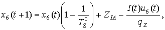
Let
![]() and
and ![]() denote, respectively,
the investment rates in industry and service. Then equations of the industrial
and service capital stocks will be:
denote, respectively,
the investment rates in industry and service. Then equations of the industrial
and service capital stocks will be:
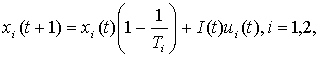 (1)
(1)
where ![]() , i=1,2, denotes,
respectively, industrial and service capital lifetimes.
, i=1,2, denotes,
respectively, industrial and service capital lifetimes.
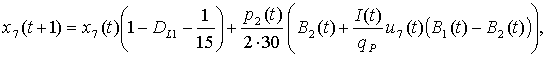
Consider
agriculture system. Let ![]() denote investment
rate in food production and let’s introduce
denote investment
rate in food production and let’s introduce ![]() as investment rate in
eroded soil restoration. Then equations for the amount of potentially arable
land and of eroded soil will be:
as investment rate in
eroded soil restoration. Then equations for the amount of potentially arable
land and of eroded soil will be:
 (2)
(2)
 (3)
(3)
where ![]() = const denotes
recovery value of 1 hectare of land.
= const denotes
recovery value of 1 hectare of land.
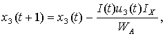
Let’s
introduce additional terms in the equations of value of nonrenewable resources
and of pollution level. They will be assigned to restoration of resources and
pollution elimination. So the equations, respectively, take the following form:
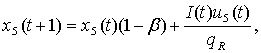 (4)
(4)
 (5)
(5)
where ![]() is investment rate in
resource restoration,
is investment rate in
resource restoration, ![]() is investment rate in
pollution control,
is investment rate in
pollution control, ![]() = const is recovery
value of one unit of pollution,
= const is recovery
value of one unit of pollution, ![]() = const is recovery value of one unit decontamination.
= const is recovery value of one unit decontamination.
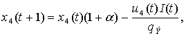
Finally,
we add one control variable ![]() to the population
system. It will denote investment rate in birth control. Then the equation of
population in the 1st age group will take the form:
to the population
system. It will denote investment rate in birth control. Then the equation of
population in the 1st age group will take the form:
 (6)
(6)
where ![]() const denotes the highest
possible budget of money for birth control.
const denotes the highest
possible budget of money for birth control.
Auxiliary
equations of the model will include the equation of inherent land fertility,
the equation of amount of urban land used, the equation of the amount of cultivated
land, the equation of population in the 3rd age group and also the
equation of total population (see [2]).
Consider
the algebraic path constraints of our model. Obviously, it will include the
following:
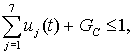 (7)
(7)
where ![]() = const denotes investment rate in the production of consumer
goods.
= const denotes investment rate in the production of consumer
goods.
Let
![]() , j = 1,…,7, designate
the minimum rate of the industrial output, assigned to each sphere at each
instant of time. Then:
, j = 1,…,7, designate
the minimum rate of the industrial output, assigned to each sphere at each
instant of time. Then:
![]() ,
, ![]() , (8)
, (8)
The
model will also include obvious nonnegativity constraints (for the pollution
level, the amount of potentially arable land, the amount of eroded soil and the
value of nonrenewable resources) and the condition, according to which the
resource restoration will not be able to give more resources than nature. Thus,
the model will contain the following algebraic path constraints:
![]() ,
, ![]() ,
, ![]() ,
, ![]() . (9)
. (9)
There
should be at least three cost functional in the obtained problem [3]. In the
environmental sphere it will be logical to minimize the pollution level. The
cost functional in the economic sphere will be defined as the production costs
to minimize. Finally, in the social sphere it is acceptable to consider the
prosperity index (introduced above), which should be maximized as the cumulated
measure of the service level. Thus, the model will include the following three
cost functionals:
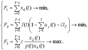 (10)
(10)
There
also will be present boundary conditions for all the seven states in the model.
Thus, the built model is a discrete-time optimal control problem with many cost
functionals, where (1) – (6) are the equations of motion (dynamic constraints),
(7) – (9) are the algebraic path constraints, (10) is the vector cost
functional.
IV. Trajectory
Optimization
In
order to prove the necessary condition for an optimal trajectory in (1) – (10)
(with boundary conditions) we use Pontryagin's maximum principle.
We
use the weighted-sum method for solving the given multi-criteria problem. Let ![]() denote the
weighted sum of F1, F2, F3 with the weights
denote the
weighted sum of F1, F2, F3 with the weights ![]() ,
, ![]() ,
, ![]() respectively.
respectively.
Rewrite
equations (1) – (6) in the following unified form:
![]() . (11)
. (11)
Since
sets ![]() , where U is the set of
admissible values of the control variables, are convex, the function f 0(x,u) is linear in u, then optimal control u* will maximize the Hamiltonian:
, where U is the set of
admissible values of the control variables, are convex, the function f 0(x,u) is linear in u, then optimal control u* will maximize the Hamiltonian:
![]() , (12)
, (12)
in u(t)ÎU, t = 0,…,T – 1, where ![]() denotes the scalar product
of the vectors
denotes the scalar product
of the vectors ![]() and
and ![]() and
and ![]() is the
solution of the costate equations.
is the
solution of the costate equations.
H is linear in u (t)
= ![]() , t = 0,…, T – 1, therefore it will attain a
maximum on the edge of the polytope, defined by U(t). Concrete values of uj*(t) can be found by comparing values at the vertices of this
polytope, using simplex method.
, t = 0,…, T – 1, therefore it will attain a
maximum on the edge of the polytope, defined by U(t). Concrete values of uj*(t) can be found by comparing values at the vertices of this
polytope, using simplex method.
The
vector x(t) will be then defined from (11) by substitution of the obtained u*(t).
![]() (13)
(13)
Since
the considered system (1) – (6) is linear (both in x and u) then
discrete-time Pontryagin's maximum principle provides also sufficient
conditions for an optimum. Thus, we have proved the following theorem.
Theorem Control
u* is optimal in (1) – (10) if and
only if it maximizes the Hamiltonian (12), t
= 0,…,T – 1, where ![]() , j=1,…,7, are
evaluated by the following formulas:
, j=1,…,7, are
evaluated by the following formulas:
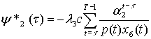 ,
,
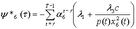 ,
,
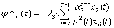 ,
,
![]() ,
, ![]() .
.
Thus,
we obtained necessary and sufficient test for optimality of trajectories for
the model (1) – (10).
References
1.
Brundtland, G.
H. (ed.), Our Common Future: World Commission on Environment and Development.
Oxford: Oxforn University Press, 1987.
2.
Chernova, E.
S., Vychislenie optimal'noj traektorii v modeli ustojchivogo razvitija regiona,
postroennoj v forme modificirovannoj global'noj modeli «Mir-3». In Bulletin of Kemerovo State University, №
2, Kemerovo, 2009, pp.48–51.
3.
Danilov, N.
N., Ustoichivoe razvitie: metodologiya matematicheskikh issledovanii. In Bulletin of Kemerovo State University.
Matematika, vyp. 4, Kemerovo, 2000, pp. 5–15.
4.
Danilov-Danil’yan,
V. I., Losev, K. S., Reyf, I. E., Sustainable Development and the Limitation of
Growth: Future Prospects for World Civilization. Berlin: Springer, 2009.
5.
Egorov, V.
A., Kallistov, V. N., Mitrofanov, V. B., Piontkovskij, A. A., Matematicheskie
modeli global'nogo razvitija. Leningrad: Gidrometeoizdat, 1980.
6.
Forrester, J.
W., World Dynamics. Cambridge, Mass: Wright-Allen Press, 1971.
7.
Herrera, A.
O., Scolnik, H. D., Chichilnisky, G., Gallopin, G. C., Hardoy, J. E., Mosovich,
D., et al., Catastrophe or New Society? A Latin American World Model. Ottawa:
International Development Research Centre, 1976.
8.
Hersh, M. Mathematical
modelling for sustainable development. Berlin: Springer, 2005, pp. 75-529.
9.
Koptjug, V.
A., Na puti k ustojchivomu razvitiju civilizacii. In Svobodnaja mysl', №14, Moscow, 1992, pp. 3–16.
10.
Meadows, D.
H., Behrens III, W. W., Meadows, D. L., Naill, R. F., Randers, J., and Zahn, E. K. O., The Dynamics of Growth
in a Finite World. Cambridge, Mass: Wright-Allen Press, 1974.