EXPERT SOFTWARE FOR IMPROVING NONCONVENTIONAL PROCESSING PARAMETERS

Tiberiu Mariu KARNYANSZKY

Dan Laurenţiu LACRĂMĂ

Faculty of Computers and Applied Computer Science

“Tibiscus” University of Timisoara, Romania

ABSTRACT

This paper is focused on the improving of the nonconventional processing parameters using computers and expert software. All over the world the nonconventional processing is used in cases where traditional techniques is too complex or too expensive, because the steel is very hard. In such situations non conventional methods like electro erosion, electrochemical erosion, complex electrochemical erosion and laser erosion could be the solution.

KEYWORDS

complex electrochemical erosion, neural networks

1. THEORETICAL CONSIDERATIONS

In order to develop a program that automatically performs the functions’ settling of the dependence of the technological parameters on the influencing factors, we have considered the following mathematical patterns with polynomial functions. Concretely, let us consider the dependences as being of one (1, 2, 3) and two variables (4, 5) only, namely:

(1) z = a₀ +a₁ · x

(2) z = a₀ +a₁ · x + a₂ ∙ x²

(3) z = a₀ +a₁ · x + a₂ ∙ x² + a₃ ∙ x³

(4) z = a₀ +a₁ · x + a₂ ∙ y

(5) z = a₀ +a₁ ∙ x +a₂ ∙ y +a₃ ∙ x² +a₄ ∙ y² +a₅ ∙ x ∙ y

the establishing of the coefficients a₀, a₁, …being based on the smallest squares method ([1]).

2. OBTAINING THE PATTERN USING MATHEMATICAL METHODS

We have obtained the following mathematical patterns of the dependence of the EEC processing productivity (Q_p) on the current density (j) and on the relative speed between PO and TO (v_r), at the debiting of the metallic carbures using OT of OL ([2]):

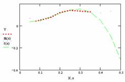
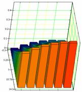
· P10 debiting (figure 1, only the dependency between Q_p and j with v_r=6):

Q_p = 0,06145 -0,9006∙j +9,55098∙j² -18,45541∙j³, error 4%

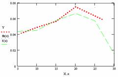
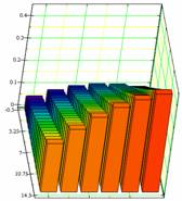
· P10 debiting (figure 2, only the dependency between Q_p and v_r with j=0.08):

Q_p = -0,06929 -0,00872∙v_r +0,00083∙v_r² -0,00002∙v_r³, error 5%

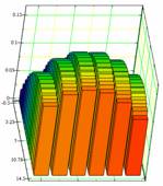
· P10 debiting (figure 3):

Q_p = -0,1376 +1,3513∙j +0,0136∙v_r -2,155∙j² -0,0004∙v_r² -0,0055∙j∙v_r, error 16,58%

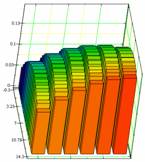
· P20 debiting (figure 4):

Q_p = -0,0674 +1,2659∙j +0,0058∙v_r -2,6495∙j² -0,0002∙v_r² +0,0130∙j∙v_r, error 9,33%

· P30 debiting (figure 5):

Q_p = -0,1168 +0,6536∙j +0,0133∙v_r +1,2880∙j² -0,0003∙v_r² +0,005∙j∙v_r, error 22.21%

· P40 debiting (figure 6):

Q_p = -0,0303 +0,2857∙j +0,0092∙v_r +0,24∙j² -0,0003∙v_r² +0,032∙j∙v_r, error 12.42%

Table 1. Experimental results – P10 debiting

j	vr	Qp	j	vr	Qp
0.08	6	0.0418	0.25	6	0.1416
	10	0.0491		10	0.1573
	15	0.0567		15	0.1805
	20	0.0752		20	0.2063
	27	0.0592		27	0.1069
0.15	6	0.0750	0.35	6	0.1253
	10	0.0930		10	0.1312
	15	0.1125		15	0.1632
	20	0.1357		20	0.1753
	27	0.0994		27	0.1156
0.20	6	0.1219
	10	0.1132
	15	0.1212
	20	0.1712
	27	0.1011

Figure 1. P10 debiting, Qp dependency on j (where Y are the experimental results, f(x) is the best approximation)	Figure 2. P10 debiting, Qp dependency on vr (Y are the experimental results, f(x) is the best approximation)

By analyzing the determined functions there can be observed that:

· the Q_p dependence on j (only) using the 3 rank functions is correct with an maximum 4% error;

· the Q_p dependence on v_r (only) using the 3 rank functions is correct with an maximum 5% error;

· the Q_p dependence on j and r_s (relative speed) using the 2 rank functions is correct with an maximum 22% error;

· Q_p can be expressed both depending on j and r_s;

· Q_p depends more on j than on r_s, both due to the 1 rank component and to the 2 rank one;

· j can be used to control Q_p better than r_s.

Figure 3. P10 debiting	Figure 4. P20 debiting

Figure 5. P30 debiting	Figure 6. P30 debiting

3. OBTAINING THE PATTERN USING NEURAL NETWORKS

In order to solve the above-mentioned task, the authors of this paper selected the Multilayer Perceptron trained with the error back propagation rule. As stated in the scientific literature MLP is a simple and powerful tool that can be applied successfully to solve many problems.

The Universal approximation theorem formulated by Cybenko proved rigorously that a single hidden layer MLP is sufficient to uniformly approximate any continuous function with support in a unit hypercube. Thus, a single hidden layer neural net should be good enough to obtain a satisfactory solution to the CEE parameters correlation problem.

Nevertheless the Universal approximation theorem has a limited practical value. The neurons inside the unique hidden layer tend to interact with each other globally. Therefore in complex situations this interaction makes it difficult to improve the approximation at a certain point without worsening it at some others. In practice, two or more hidden layers can prove useful in order to make the approximation process into a more manageable one.

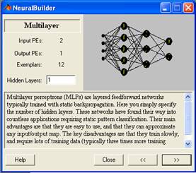
Figure 7. Neural Builder GUI window, Neuro Solutions 4.31

Consequently the authors decided to experiment and compare the results of three alternative neural architectures:

a. Single hidden layer MLP;

b. Two hidden layers MLP;

c. Three hidden layers MLP.

All the three neural nets were implemented using the Neuro Solutions 4.31 software from Neuro Dimensions Inc. This integrated environment provided us the possibility to quickly build, train and test the networks using a simple and efficient set of GUI and results windows as shown in Figure 2.1. Each of the three neural nets architecture is depicted in Figure 2.2 as shown in the Neuro Solutions user screen.

As stated before each of the three neural nets is able to assure a reasonably good approximation of the curve t_p=f(I,W_TO), but the authors tried to find out which of them is the best solution both in terms of precision and efficiency.

Input layer	Hidden layer	Output layer		The criterion
a.
Input layer	Two hidden layers	Output layer		The criterion
b.
Input layer	Three hidden layers		Output layer		The criterion
c.

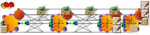
Figure 8. Neuro nets architecture

3. Experimental Results

Using the three structures represented above the authors performed the experiments with the same training set containing 388 data samples.

	Single hidden layer MLP: CV Avg. Cost @ 0.05 Training epochs @ 760
	Two hidden layers MLP: CV Avg. Cost @ 0.02 Training epochs @ 580
	Three hidden layers MLP: CV Avg. Cost @ 0.02 Training epochs @ 670

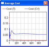
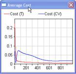
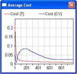
Figure 9. CV and T Average Costs

Each sample consists of the directly measured technological parameters of the debiting process on a real CEE machine tool (i.e. t_p, I and W_TO). All data were collected from the same equipment using only OL37 stainless steel samples. The data collecting procedure was made in accordance with the rules stated in [4].

The CV and T average costs together with the number of minimum necessary training epochs are shown for all the three neural nets in Figure 3.1.

The test set was the same for all the three nets and it was performed with 82 different data samples.

Table 2. experimental results with Neural Networks

Neural net Structure	Incorrect estimations
	Samples	[%]
One hidden layer	5	93.902
Two hidden layer	3	96,342
Three hidden layer	2	97.561

4. Conclusions

The most important concluding comment of the above results is that the use of neural nets produces a significant improvement from the method of curve fitting with the third rank polynomial functions. This progress was achieved without employing great programming effort or extensive time-consuming computations.

Analyzing the incorrect estimations in all the three cases some concluding remarks are obvious:

· The two hidden layers MLP is the best solution because it gives more precise results than the single hidden layer structure;

· The three hidden layers structure performs a little better at the testing stage, but the improvement is not significant and consequently the added costs are not worthwhile;

· Better results should be obtained with an enlarged number of data samples in the training set, but the data collection procedure involves a great effort and it is time consuming.

Further improvements in performance could result from using a more flexible structure as RBF neural nets. This could lead to the development of a neural network able to solve the parameters control for a set of similar but different stainless steel qualities.

The use of neural networks to manage mechanical processes parameters is a very useful practice, but finding the optimal solution is not straightforward and need a carefully work from the data collection stage to the final implementation, training and testing.

REFERENCES

[2] Tiberiu-Marius Karnyanszky, Contribuţii la conducerea automată a prelucrării dimensionale prin eroziune electrică complexă, Teză de doctorat, Universitatea “Politehnica” Timişoara, 2004

[2] Ştefan Kilyeni, Metode numerice, volumul I+II, Editura Orizonturi Universitare, Timişoara, 1997

[3] Zenoviu Lăncrăngean, Contribuţii la prelucrarea corpurilor de revoluţie prin eroziune electrică complexă, Teză de doctorat, Institutul Politehnic „Traian Vuia” Timişoara, 1986

¹ Assoc.Prof. Tiberiu Marius KARNYANSZKY, PhD., Dipl.Eng.,

“Tibiscus” University of Timisoara, Romania,

mtk@tibiscus.ro,

+40/744/599190

¹ Assoc.Prof. Dan Laurenţiu LACRĂMĂ, PhD., Dipl.Eng.,

“Tibiscus” University of Timisoara, Romania,

dlacrama@tibiscus.ro,

+40/722/329912