Natalia Ovsyannikova
Northern (Arctic) Federal University named after M.V.
Lomonosov
A stochastic model of epidemic
Determined model, describing
uncontrolled process of the spread of epidemic, is described by a system of
differential equations:
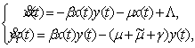 (1)
(1)
![]() ,
, ![]() ,
, ![]() ,
, ![]() ,
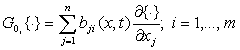
, ![]() (2)
(2)
where ![]() the rate of
change in the number of people exposed to the disease,
the rate of
change in the number of people exposed to the disease,
![]() the rate of
change in the number of infected people,
the rate of
change in the number of infected people,
![]() function characterizing the number of meetings of people exposed to the
disease and infected ones per unit of time.
function characterizing the number of meetings of people exposed to the
disease and infected ones per unit of time.
![]() - the number of people who
regained their health per unit of time without the influence of external means:
quarantine, vaccination and others (
- the number of people who
regained their health per unit of time without the influence of external means:
quarantine, vaccination and others (![]() -average time of natural healing),
-average time of natural healing),
![]() - the growth coefficient, which
characterizes the frequency of meetings of healthy people with infected people (in
general case it can be considered as a function
- the growth coefficient, which
characterizes the frequency of meetings of healthy people with infected people (in
general case it can be considered as a function ![]() ),
),
![]() - the coefficient of natural mortality of people,
- the coefficient of natural mortality of people,
![]() - the coefficient of mortality from this infection,
- the coefficient of mortality from this infection,
![]() - average birthrate (reproduction).
- average birthrate (reproduction).
The considered
mathematical model is determined and allows to calculate in advance the change
of a condition of the studied system, on an interesting time segment by solving
the Cauchy problem (1)-(2). We can
assume that the values of some of the coefficients of the system
in the moment (of time) ![]() are not uniquely defined, for
example, because of their dependence on many unpredictable factors, and they
can be regarded as random processes, the mathematical expectations of which are
known.
are not uniquely defined, for
example, because of their dependence on many unpredictable factors, and they
can be regarded as random processes, the mathematical expectations of which are
known.
Assume that the
coefficient of growth has a random component![]() , i.e. it can be represented as:
, i.e. it can be represented as:
![]() , (3)
, (3)
where ![]() - mathematical expectation
(mean) of the coefficient
- mathematical expectation
(mean) of the coefficient ![]() , set it permanent, i.e.
, set it permanent, i.e. ![]() ;
; ![]() - random process;
- random process; ![]() - constant characterizing the
degree of influence of the random perturbation on the value of the coefficient
- constant characterizing the
degree of influence of the random perturbation on the value of the coefficient![]() .
.
In this case, the
mathematical model (1)-(2) takes the following form:
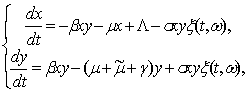 (4)
(4)
![]() (5)
(5)
In this case, the
state of the system![]() is no longer a deterministic vector-function but is a vector random
(stochastic) process
is no longer a deterministic vector-function but is a vector random
(stochastic) process![]() ,
, ![]() .
.
In general (in a
general view), the system (4)-(5) can be written:
![]() (6)
(6)
![]() , (7)
, (7)
where ![]() ;
; ![]() ;
; ![]() - scalar Wiener
process;
- scalar Wiener
process; ![]() ,
, ![]() ,
, ![]() ,
, ![]() .
.
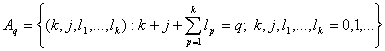
The obtained
stochastic differential equation will be solved numerically, for this we use a
stochastic analogue of Taylor's formula. Apply the unified stochastic Taylor-Ito
expansion in iterated stochastic integrals and also the approximation of
iterated stochastic integrals by means of the polynomial system of functions.
[1]
Formulate a theorem
on Ito process expansion (decomposition) ![]() , where R:
, where R:![]() , in the unified Taylor-Ito series in
iterated stochastic integrals
, in the unified Taylor-Ito series in
iterated stochastic integrals![]()
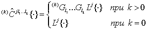
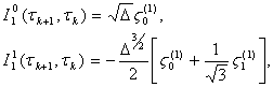
Theorem 1. Let the
process ![]() be Ito continuously
differentiable
be Ito continuously
differentiable ![]() times in the
mean-square sense on
times in the
mean-square sense on ![]() along
trajectories of the equation (6). Then for all
along
trajectories of the equation (6). Then for all![]() ,
, ![]() it decomposes
into a unified Taylor-Ito series of the following
it decomposes
into a unified Taylor-Ito series of the following 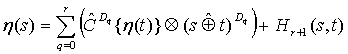 type:
type:
(8)
and there exists such a
constant ![]() that
that
![]() ,
, ![]() ,
,
where ![]() , (9)
, (9)
 , (10)
![]() , (11)
, (11)
![]() , (12)
, (12)
![]() (13)
(13)
 , (14)
![]() , (15)
, (15)
![]() , (16)
, (16)
![]() , (17)
, (17)
 (18)
(18)
 ,
(19)
,
(19)
 , (20)
 , (21)
equality (8) is
just(is fair, is true, takes place, holds) with probability 1, right parts of (8)-(10)
exist in the mean-square sense.
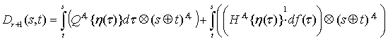
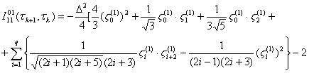
We construct a
unified Taylor-Ito expansion for the components of the solution ![]() of the system (4)-(5) for
infinitesimal of order of
of the system (4)-(5) for
infinitesimal of order of ![]() , i. e. we will construct expansion of Ito process
, i. e. we will construct expansion of Ito process ![]() :
:
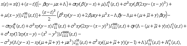 (22)
(22)
 (23)
(23)
Relations (22) - (23) on a uniform discrete grid ![]() constructed for the
segment
constructed for the
segment ![]() , such that
, such that ![]() ,
, ![]() are selected as a numerical method for modeling the
system (6)-(7). Denote
are selected as a numerical method for modeling the
system (6)-(7). Denote ![]() ,
, ![]() , and then by putting
, and then by putting ![]() ,
, ![]() ,
, ![]() in
expansions (22)-(23) and using the expansions
of the iterated stochastic integrals
in
expansions (22)-(23) and using the expansions
of the iterated stochastic integrals ![]() in terms of a polynomial basis, the
following expressions for the numerical method are obtained:
in terms of a polynomial basis, the
following expressions for the numerical method are obtained:
 (24)
(24)
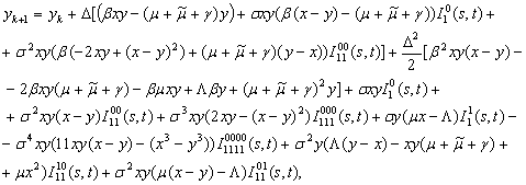 (25)
(25)
where
![]()
![]() (26)
(26)
![]()
![]()
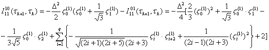
![]() - a
system of independent Gaussian random variables with zero mean (expectation)
and variance of one, which is generated on a step of integration with a number
of k and is independent with the analogous systems of random variables that are
generated on all the preceding steps of integration towards (with respect to)
the step of integration with the number of k;
- a
system of independent Gaussian random variables with zero mean (expectation)
and variance of one, which is generated on a step of integration with a number
of k and is independent with the analogous systems of random variables that are
generated on all the preceding steps of integration towards (with respect to)
the step of integration with the number of k; ![]() - step
of integration of the numerical method; the number
- step
of integration of the numerical method; the number ![]() is chosen from the condition ([1], p.199):
is chosen from the condition ([1], p.199):
 (27)
(27)
where constant ![]() must be given (set). We choose it for the sake of simplicity to be
unity (to be equal to one). The value of
must be given (set). We choose it for the sake of simplicity to be
unity (to be equal to one). The value of ![]() increases with a decrease in the value of the step of integration.
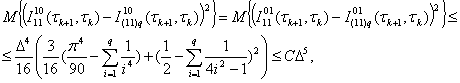
Consider the results of the choice of number
increases with a decrease in the value of the step of integration.
Consider the results of the choice of number ![]() with
the help of the relation (13). These results are placed in the following table:
with
the help of the relation (13). These results are placed in the following table:
|
|
0,004 |
0,001 |
0,0005 |
|
Q |
1 |
2 |
4 |
I. e., it is enough
to let q be equal to 1 that ![]() would
be 0,004, then the expansions for
would
be 0,004, then the expansions for ![]() and
and ![]() take the form:
take the form:
![]()
![]()
Make the numerical modeling of the solution of the system (6)-(7) by means of relations (24)-(25) on the time
interval Т=10 with the step ![]() with
the following initial data:
with
the following initial data: ![]()
![]()
![]()
![]()
![]()
![]() . The result of the numerical modeling is
presented on fig. 1. Now introduce the stochastic perturbation
. The result of the numerical modeling is
presented on fig. 1. Now introduce the stochastic perturbation ![]() . The evolution of processes
. The evolution of processes![]() , which characterize the process of evolution
of epidemic of the system (6)-(7) for values
, which characterize the process of evolution
of epidemic of the system (6)-(7) for values ![]() is presented on figs. 1-4 respectively. The values of the maximal trajectories
deviations of the perturbed system from the trajectories of the determined
system are listed in table 1, from which direct dependence of maximal
deviations of the solution of a perturbed system on the value of the perturbed
parameter
is presented on figs. 1-4 respectively. The values of the maximal trajectories
deviations of the perturbed system from the trajectories of the determined
system are listed in table 1, from which direct dependence of maximal
deviations of the solution of a perturbed system on the value of the perturbed
parameter ![]() is well
seen.
is well
seen.
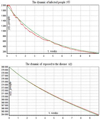
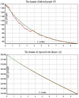
Fig.1
Determined and stochastic models Fig.2 Determined and stochastic models
of epidemic (![]() ) of epidemic (
) of epidemic (![]() )
)
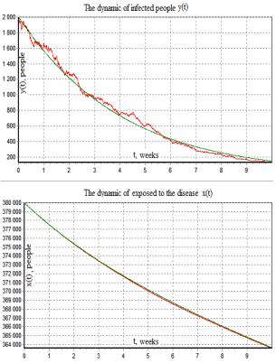
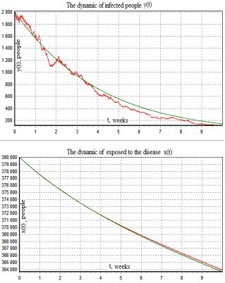
Fig.3 Determined and
stochastic models Fig.4 Determined and stochastic models
of
epidemic (![]() ) of epidemic (
) of epidemic (![]() )
)
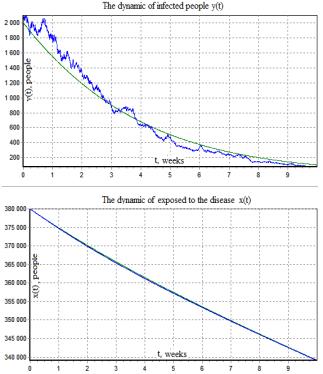
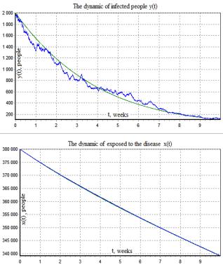
Fig.5 Determined
model and mean of the solution of Fig.6 Determined model and mean of the solution
of
system (6, 7) found in 5 realizations (![]() ) system (6, 7) found in 10 realizations (
) system (6, 7) found in 10 realizations (![]() )
)
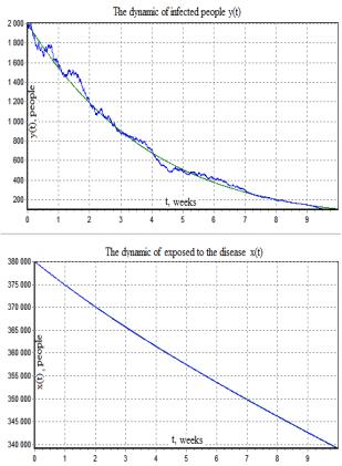
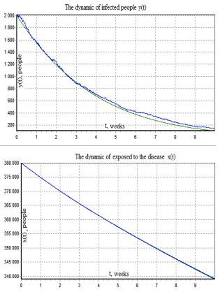
Fig.7 Determined
model and mean of the solution of Fig.8 Determined model and mean of the solution of
system (6, 7) found in 15 realizations (![]() ) system
(6, 7) found in 50 realizations (
) system
(6, 7) found in 50 realizations (![]() )
)
Table
1
|
Value of |
Maximum deviation of the trajectories of the perturbed system from
the trajectories of the determined system depending on the value of the s. |
|
|
Deviation X, % |
Deviation Y, % |
|
|
|
Practically none |
2,5 |
|
|
Practically none |
3,5 |
|
|
0,1 |
4 |
|
|
0,12 |
4,5 |
|
|
0,15 |
5 |
For σ≤![]() stochastic model is almost equal to the
determined one, so it is necessary to take the determined model for description
of the system; for σ>
stochastic model is almost equal to the
determined one, so it is necessary to take the determined model for description
of the system; for σ>![]() the stochastic model significantly (by more than 5%) is different from the determined one;
therefore the perturbed coefficient needs to be taken ranging from
the stochastic model significantly (by more than 5%) is different from the determined one;
therefore the perturbed coefficient needs to be taken ranging from ![]() to
to ![]() .
.
For different
realizations of the system of independent Gaussian values ![]() we
obtain different realizations of the solution of the system of stochastic
differential equations (6). These
trajectories for small perturbations lie inside of a tube constructed in a
small neighborhood of the solution of determined system (1). Find mean of the solution
of system (6) in 5, 10 realizations for
we
obtain different realizations of the solution of the system of stochastic
differential equations (6). These
trajectories for small perturbations lie inside of a tube constructed in a
small neighborhood of the solution of determined system (1). Find mean of the solution
of system (6) in 5, 10 realizations for ![]() , in 5, 10, 15 and 50 realizations for
, in 5, 10, 15 and 50 realizations for ![]() . On figs. 5-8 it is shown a comparison of
means with the solution of the determined system of differential equations (1).
One can conclude that
. On figs. 5-8 it is shown a comparison of
means with the solution of the determined system of differential equations (1).
One can conclude that ![]() , which is confirmed by numerical experiments,
where
, which is confirmed by numerical experiments,
where ![]() - solution of determined system (1), (2),
- solution of determined system (1), (2), ![]() -
solution of stochastic system (4), (5).
-
solution of stochastic system (4), (5).
References:
1.
Kuznetsov D. F. Numerical modeling of
stochastic differential equations and stochastic integrals St. Petersburg:
Science, 1999, 459s.
2.
Dmitrieva O.N. A stochastic model of the
dynamics of the forests.- Collection of proceedings - Tver, 2006, 187 p.