Advanced Information Technologies/4

Advanced Information Technologies/4. Information security

associate professor Karpinets V., Kets D., Kravets S.

Vinnitsya National Technical University, Ukraine

Analysis of self-similarity high traffic packet data channel

Introduction

The end of XX – the beginning of the XXI century were marked by revolutionary changes in telecommunication area. The theory of convergence formulated by the end of the 90th years of the XX century, practically found at once the realization and as the result of this realization happens today radical changes in various types of services and telecommunication technologies.

Existence of a large quantity of diverse services in one physical channel at o'clock of the highest loading can lead to an overload of switching and Terra line devices on the main communication lines and as a result to partial or complete degradation of network infrastructure and refusal of a wide range of provided services. For prevention of situations of leaders to refusal of the main network equipment of the most significant, become a problem of engineering of a traffic. It is obvious that the problem of traffic control is necessary not only for prevention of possible overloads in a network, but also for optimization of use of network resources for extraction of the maximum profit at the minimum utilization of a communication channel. Thus, capacities of the main and sub main channels should be enough not only for existing network services, but also for development and introduction of new network services, providing thus necessary quality of delivery.

Experiment technique

Experiment on research of statistical characteristics of a traffic of a network was put as follows. In a network of the city the switchboard providing translation of the maximum volume of a traffic was chosen. The personal computer (personal computer) was connected to free port of the switchboard on the RJ-45 interface with measuring ON. At channel level, communication was carried out according to the Gigabit Ethernet protocol. The chosen port of the device was configured in the form of the SPAN port, specularly displaying the data entering into the switchboard, i.e. the simplex Rx-channel. As measuring ON the program sniffer developed by the author based on open library WinPcap with use of the timer of high resolution was used. The software allows to fix an event of arrival of a package to within 10 nanoseconds. After capture of hundred million frames the sniffer stopped and made data processing, bringing the received realization into an equidistant form with a constant step of m by means of aggregation procedure, and then repeatedly made capture of a traffic and the analysis of data. Time of the beginning of capture of a traffic 07:41:16.05.2009, and the general time of measurement made 3:08:54 PM. Thus, 18 profiles of a network traffic were received. The logic scheme of the organization of a network is displayed in the Fig. 1.

Calculation of the minimum interframe interval in the Gigabit Ethernet standard makes 608 nanoseconds [1]. The minimum frame of Gigabit Ethernet consists of a preamble (serves for transmitter and receiver synchronization at physical level), the office part, useful loading, a field of control sequence of a frame and a field of expansion bearing.

Figure 1 – the Logic scheme of the organization of monitoring of a network traffic

The size of a preamble is fixed and makes 64 bits, an office part in 144 bits, useful loading in 368 bits, control sequence in 32 bits, and the field of expansion of the bearing supplements the size of a frame to 512 bits. The minimum value of a "pure" interframe interval is equal in accuracy to time of transfer of 96 bits and makes for Gigabit Ethernet of 96 nanoseconds, and the maximum value is not limited. Considering that the preamble at channel level is not processed, we receive value of a "real" minimum interframe interval in 608 nanoseconds. It testifies that the chosen interval scale in 10 nanoseconds, the developed program sniffer, is capable to distinguish two consistently coming frames.

The analysis of the received data

For research of structure of a traffic and an illustration of its fractal (self-similar) character the mathematical Matlab package was used. As a result of process of aggregation of profiles of a network traffic temporary ranks were received. Examples of profiles of byte intensity, and also intensity of packages in unit of time, are given on (the Fig. 2). Process of aggregation was made in compliance with a technique offered in [2] on a formula:

where – counting number in the received profile;

m – the size of the block or time interval aggregations;

k – block number.

Each point on this schedule represents number of bytes of information transferred in the main channel for an interval of time in 0,001 second. Duration of this realization makes 1461867 points or 24 minutes and 21 seconds. As result to transfer such traffic without loss, capacity of the channel should correspond to level of peak emissions, i.e. in this case to be not less than 3668800 Bits/ms.

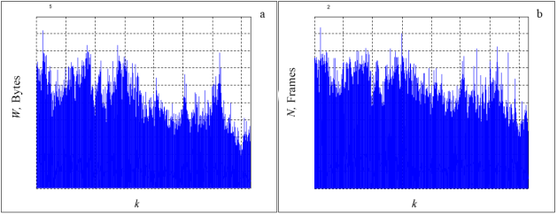
Figure 2 – the Measured realization: a) byte intensity; b) intensity of packages

The visual analysis of histograms of distribution of lengths of frames shows (the Fig. 3) that in a network frames in the size of 1518 bytes, i.e. the maximum size of a frame supported by the Ethernet technology prevail.

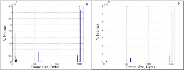
Figure 3 – Histograms: а) distribution of lengths of frames, b) distribution of number of data transferred by frames of the corresponding length

It is obvious that for practical purposes information on degree of load of a network is more useful. Information on quantity of packages in unit of time can visually mislead, as at a network there can be many small managing directors of the packages which are not bearing useful information, and packages of the minimum length which create the peaks incoincident with peaks of byte speed.

The statistics of the received realization is given in Tab. 1. From the table it is visible that during creation of profiles of a network traffic it was transferred 1.54 Tbyte of data 75.33 % on the average from which were transferred by a frame of the maximum size, and 0.0044 % of data were on the average transferred by a frame of the minimum size. In the provided table also can cause interest a traffic profile at number 16 which has the minimum percent of data transferred a frame in the size of 1518 bytes. It is possible to explain it to that data were transferred in this time period mainly by the frames which length is distinct from the considered.

Table 1 - Statistics of distributions of lengths of frames

№	Realization name	Number of data transferred a frame in the size of 64 bytes, Byte	Number of data transferred a frame in the size of 1518 bytes, Byte	In total transferred data, Byte	Percent of data transferred a frame in the size 64 bytes from all transferred data, %	Percent of data transferred a frame in the size of the 1518th byte from all transferred data, %
1	07.41.16.05.10.09	2084352	80087938388	94182789518	0.0022%	85.0346%
2	39.17.17.05.10.09	1596992	75781109522	96592015584	0.0017%	78.4548%
3	20.47.17.05.10.09	1770816	62788527758	81889732017	0.0022%	76.6745%
4	33.20.18.05.10.09	1813376	78568949758	94668673869	0.0019%	82.9936%
5	44.54.18.05.10.09	2029504	71497815786	87749499857	0.0023%	81.4795%
6	35.25.19.05.10.09	1653056	62512934338	81533283187	0.0020%	76.6717%
7	06.57.19.05.10.09	1717504	64159153472	83324079817	0.0021%	76.9995%
8	30.30.20.05.10.09	1506432	73557785382	88694541378	0.0017%	82.9338%
9	48.58.20.05.10.09	1625088	65226962532	84078551606	0.0019%	77.5786%
10	51.30.21.05.10.09	1518912	67350417176	87890062866	0.0017%	76.6303%
11	39.00.22.05.10.09	1720128	66441331334	85141916508	0.0020%	78.0360%
12	42.31.22.05.10.09	1854400	67204367652	87147616740	0.0021%	77.1156%
13	19.06.23.05.10.09	2289792	64344943982	80737410877	0.0028%	79.6966%
14	13.45.23.05.10.09	4077824	53103018586	77754997124	0.0052%	68.2953%
15	19.52.00.06.10.09	6315328	49301555350	84050882091	0.0075%	58.6568%
16	49.34.02.06.10.09	1938137	35877170188	73215120704	0.0265%	49.0024%
17	43.40.07.06.10.09	7658432	74421216554	95619080236	0.0080%	77.8309%
18	58.03.10.06.10.09	4934272	60459594548	84147015412	0.0059%	71.8500%
Total:		65547584	1172684792306	1548417269391	0.0044 %	75.3297 %

It is known that self-similar processes with H from 0.5 to 1 possess property of the long-term dependence (LTD), i.e. their autocorrelation function (AСF) does not agree on infinity to zero. Thus, it is necessary to solve a problem of regression and to calculate on experimental AСF a method the smallest squares model (1) and parameters.

At creation of autocorrelation function the first 200 delays were considered (Fig. 4).

$C:\Users\Sergey\Desktop\Снимок.PNG$

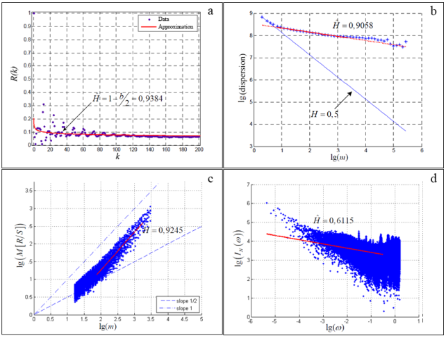
Figure 4 – Schedules of an assessment of an indicator of Hurst: а) factor of correlation from a delay; b) dispersion change; c) R/S - statistics; d) periodogram method.

The analysis of change of dispersion (the Fig. 4) is based on property of slowly fading dispersion of self-similar processes at association (aggregation) (1). According to it dispersion united (precisely or approximately) self-similar process satisfies dependences

where - the parameter connected with by a ratio .

At process aggregation with various levels of m dispersion usually fades very quickly (H = 0,5). Exceptions make self-similar processes, for which dispersion fades slowly, under the sedate law (at great values of H).

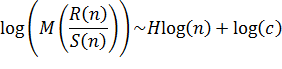
Taking the logarithm both parts of a ratio (3) for the incorporated dispersion, we will receive expression

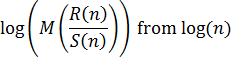
Apparently, the assessment of can be received calculation for various values , displaying results from and having carried out a straight line on a method of the smallest squares through the received points.

For detection of self-similarity in time series often resort to R/S to statistics (Fig. 4, c). In practice it is convenient to use expression

Having used this expression, it is possible to estimate H, having represented the dependence diagram

Selecting a straight line for a method of the smallest squares to R/S-diagram points, on an inclination of the line of regression find an assessment for H.

The considered methods of an assessment of an indicator of Hurst of H are not too exact and state only an assessment of level of self-similitude in a time series. Therefore, whether this method can be used only to test a time row is self-similar, and if is, to receive a rough estimate of H.

Assessment of an indicator of Hurst based on graphics of spectral density. (Fig. 4, d), makes an essence of a method which provides big statistical severity, than estimates based on association. However, the price of existence of a parametrical method is the requirement that the parametrical model of process was known in advance. Periodogram estimates spectral density of discrete stochastic process of t and it can be estimated by a row (4) on an interval of time of :

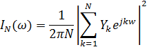
where – a time row; N – length of a time series.

Considering, what self-similitude influences character of a range of at , should be the diagram of dependence of spectral density of a look will turn out

Having constructed the diagram only for low frequencies select a tangent a straight line to a curve. The inclination of the line will be approximately equal 1-2H. It is important to note that H approach to 1 says about high self-similitude of this process and that the behavior of process is persistent or process possesses long memory. That is, if on some temporary interval in the past the positive increment of process was observed, in other words, the increase, and in the future will occur on the average increase.

At H=0.5 the process deviation from an average is casual and does not depend on the previous values.

At 0<H<0.5 process is changeable, i.e. increase relatively average in the past, in the future will be replaced in an opposite direction.

To avoid difficult tests for check of a stationarity it is possible to use the following method. Let's estimate Hurst's indicator for blocks of data of D. Let's consider K of segments of the row, everyone long N. Hurst's indicator of H is estimated in each segment with use, in our case, RS-the analysis, the analysis of change of dispersions, the periodogram analysis and AKF analysis. In [8] it is in detail stated advantages and shortcomings of methods used in this article. If estimates in i-block are designated as by , when for the corresponding N can be found an assessment of an indicator of Hurst in a look

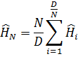
Thus, if to choose N rather big, it is possible to provide acceptable convergence of an assessment so that for stationary process an assessment did not depend on N. As a result, the following estimates of an indicator of Hurst of H (Tab. 2) were received.

Table 2 – Assessment of an indicator of Hurst various methods

№	Realization name	Method of an assessment of an indicator of Hurst
№	Realization name	RS-statistics	Periodogram	Dispersion changes	AKF
1	07.41.16.05.10.09	0,9062	0,6690	0,9597	0,9534
2	39.17.17.05.10.09	0,9116	0,6744	0,9389	0,9211
3	20.47.17.05.10.09	0,9245	0,7138	0,9560	0,9476
4	33.20.18.05.10.09	0,9477	0,5874	0,9379	0,9348
5	44.54.18.05.10.09	0,9031	0,7014	0,9496	0,9356
6	35.25.19.05.10.09	0,8955	0,6358	0,9188	0,9255
7	06.57.19.05.10.09	0,8731	0,6829	0,9058	0,9205
8	30.30.20.05.10.09	0,8576	0,6706	0,9142	0,9110
9	48.58.20.05.10.09	0,9643	0,6900	0,9466	0,9344
10	51.30.21.05.10.09	0,8911	0,6794	0,9129	0,9083
11	39.00.22.05.10.09	0,8987	0,6998	0,9062	0,9152
12	42.31.22.05.10.09	0,9418	0,7108	0,9233	0,9284
13	19.06.23.05.10.09	0,9369	0,7191	0,9545	0,9511
14	13.45.23.05.10.09	1,0475	0,7050	0,9645	0,9816
15	19.52.00.06.10.09	1,0284	0,7263	0,9820	0,9629
16	49.34.02.06.10.09	1,0144	0,7286	0,9514	0,9797
17	43.40.07.06.10.09	1,0609	0,7154	0,9761	0,9715
18	58.03.10.06.10.09	0,9990	0,7308	0,9606	0,9506
		0,9446	0,6911	0,6911	0,9422
SD		0,0614	0,0360	0,0360	0,0237

Conclusion

Modern networks - networks with a wide set of every possible services and services. A part from them are services of a time-dependent traffic (the IP-telephonies services, streaming video, different types of scheduling of the equipment), other part, for example, file exchange networks of FTP servers are not critical to the current capacity. The special attention is deserved by services of the distributed data storage of P2P. Universal distribution of this type of service, absence of «a narrow throat» as the element of system limiting total amount of being broadcast data allow to consider further development of the P2P networks as a factor bringing an imbalance in existing network infrastructure [8].

Today with emergence broadband network services, problems of improvement of quality of service, long-term forecasting of loading of communication channels, the engineering and management of a network become more and more actual.

List of references

1. Norris, M. Gigabit Ethernet/M. Norris//Technology and Applications. - Artech House, 2003.

2. Petrov, Century of Century. Statistical analysis of network traffic / Century. In Petrov. - Moscow, 2003.

3. Shelukhin, O.I.Samopodobiye and fractals. Telecommunication appendices / Lakes. I.Shelukhin, A.V.Osin, Page. M Smolsky. - M: Physlit, 2008.

4. Y.A. Razrabotka's hooks of the program focused multi-purpose network of the distributed calculations of scale of the small city: Cand.Tech.Sci. / Yu.A.Kryukov. - Dubna, 2004.

5. Karagiannis, T. POISSON VIEW OF INTERNET TRAFFIC/T. Karagiannis, M. Molle, M. A. FALOUTSOS//NONSTATIONARY INFOCOM 2004. Twenty-third AnnualJoint Conference of the IEEE Computer and Communications Societies, March 2004. - vol.3, issue, 7-11. - P. 1558-1569.

6. Afontsev E.V., Development of a technique of detection of anomalies of a traffic in the main Internet channels. Dissertation, 2007.

7. Hurst, H. E. Long-term storage capacity of reservoirs. Trans. Am. Soc. Civil Engineers. - 116:770-799, 1951.

8. O Rose., Estimation of the Hurst Parameter Time Series. 1996.