http://www.rusnauka.com Mathematics/5. Mathematical modelling

Karvatskiy A.Ya., Dudnikov P.I., Leleka S.V., Shilovich I.L., Pulinets I.V.

National technical university of Ukraine

“Kiev polytechnic institute”

To the consideration of radiation and complicated heat transfer problem solution by boundary elements method

Most of the problems which can be reduced to tasks of radiation heat exchange (further – radiation) between solid bodies of the complete shape divided diathermic environment, have no direct analytical decision. Usually for such tasks solution numerical methods are used: zonal, Monte-Carlo [1], traces of rays [2,3]. However the method of boundary elements (BEM) can be effectively applied to problems with diffuse borders [4,5]. Complex heat exchange problems solution, for example, stationary radiating and conductive heat transfer, without and with interaction between bodies are most interesting in practice. Technique of numerical solution of the conductive heat exchange problem on the basis of BEM is described in [6]. To solve the radiating heat-conduction problem and complex heat exchange effectively it is necessary to solve some problems connected with: calculation of radiation influence factors for diathermic cavity surrounded by non-transparent (opaque) diffused - reflecting borders; taking into account effect of beams shielding at influence factors calculation; joint solution of the nonlinear equations system which describe conductive and radiation heat transfer. This work main objective is to develop the BEM numerical technique and work out a software for solution of radiating and complex heat exchange problems.

Let's consider problem statement as follows. Let is the area which includes an ensemble of (some industrial equipment elements of construction) boundary lines of which are a conjugation of piecewise - flat ensembles . So at means a solid heat-conductive bodies, and at - diathermic cavities between boundaries of which the radiation heat transfer has take place. In solid heat conductors bodies for the account of boundary line the solid - melt is used the generalized statement of problem. On boundary lines of a construction with 3-rd types of boundary conditions (BC), and on - a union of contacts between various members are observed. As on are set various BC it also can be presented in the form of unions: , where - BC of Dirichle, - BC of Neumann, - BC the convective type. To take into account solid-melt border in solid heat conductors a generalized problem statement is used.

In the case of outer boundary with 3 types of boundary conditions (BC) a definition of is applied, in the case of - contacts joining between different elements is considered.

As at a different BC are applied it could be considered as unification: , where - BC Dirichle, - BC of Neumann, - BC of convective type. Due to the existing of radiation heat transfer a is considered as unification: , where - surface contacts between heat conductors , - surface contacts between diathermic or transparent solid and non-transparent solid heat conductors.

On the base of written previously, with accounting of complete heat transfer a temperature field in could be described by next equations set with correspondent BC:

(1)

(2)

(3)

(4)

where - heat conductivity, Wt/(m×К); - temperature, К; - Hamiltonian; - Cartesian coordinates, m; - intensity of the heat internal source in , Wt/m³; - Stephan-Boltsman constant, Wt/(m²×К⁴); F - diathermic area surface; - distance between points x and y, laying on surfaces F, m; - surface emissivity F; - corners between normals to surface F in points x, y and a vector , rad; q_r - radiant flux density, Wt/m²; - temperature of crystallization, К; - an interval of smoothing, К; - an external normal to border ; - effective heat-transfer coefficient, Wt/(m²×К); – temperature of environment, К; , – values of function on the right and to the left of , К; ; – vector of heat-flux density by conductivity, Wt/m²; – total heat flux density in diathermic medium, Wt/m²; – total heat flux density in transparent medium, Wt/m²; – total heat flux density in non-transparent medium (heat conductivity medium), Вт/м²;- solid-melt joint space (area); – areas (elements of construction) number;

.

So the system of the integro-differential equations (1) together with BC (3), (4) is the full mathematical formulation of assigned problem.

As numerical solution of a heat equation technique is described enough in [6], we shall restrict our analysis by consideration of the solution of integrated equation of system (1) technique. First of all we shall execute some transformations. To do this the system (1) of integrated equation of radiation heat transfer has to be written in a digital form on conditions that on the G_j values of T⁴, q_r are accepted constants

, (5)

where H and G – influence factors for temperature and radiant heat-flux density; N – number of nodes on boundary G; i – index of a source; j – index of a current node; G_j – element of discretization G;

, (6)

, (7)

- Kronecker symbol.

Assume that emissivity does not depend from x, so on G_j. Such assumption allows to simplify and to eliminate considerably a number of H and G calculations.

Then expression (7) transfers to

(8)

To take into account (8) influence factors equation will be presented as

, (9)

, (10)

where. (11)

So a influence factors calculation is reduced to only one integral (11). Equations (9) and (10) are available for the single nodes at linear elements (or for constant elements). At double nodes the situation is quite different:

, (12)

. (13)

Equations (12) and (13) are available both for double nodes as well as for single nodes. However, at the single or central nodes is accepted, that

, therefore it is available .

The order of h_ij calculation depends on a type of boundary elements obtained as a result of digitization of a boundary surface. For boundary elements we shall choose triangular linear elements [6]. Thus numbering of tops of the triangles limiting the node j, is carried out so that the top conterminous with the node j, had number 3, in each of the specified triangles.

Let's enter function

.

In each triangle function changes under the linear law, for example, for F and q_r will be

(14)

coordinates

where indexes 1,2,3 – relate to numbers of tops of triangles; – oblique coordinates.

To keep the form of the boundary equations BEM (5) together with using of (9), (10), we shall write down h_ij relate to nodal surface points j. In this case the coefficientт h_ij even at use of linear elements becomes independent from function or a stream and can be calculated beforehand. According to [6] it is obtained

, (15)

where L – quantity of triangles, limiting the node j; k – index of triangles.

Let's substitute from (11) into (15), we'll get

,(16)

where ; – Jacobian;

, (17)

, (18)

To take into account of (17) and (18) for (16) we'll get

(19)

The integral (19) can be defined numerically with the using of Hamer’s quadrature [5]

, (20)

where – nodes and weights of quadrature on a simplex; n – quantity of nodes of quadrature; n_x, n_y, n_z – directional cosines an external normal to a plane [6]; – coordinates of nodes [6].

How to definite . Let’s in space there is a triangle with vertexes and a vector with terminuses and (fig. 1). It is necessary to define conditions at which vector crosses an interior of a triangle .

Assumption 1. Points 1, 2 and 3 don't lie on one straight line.

Conditions of check

or .

The assumption 2. Points А and В lay on the different sides from a plane in which the lays.

Terms of verification

.

Fig. 1. The scheme for calculation

At the given assumptions vectors , и create basis of space . Let's perform a vector as linear combination of vectors

, and :

. (21)

Than a vector crosses an interior of a triangle if and only if, when

. (22)

Let's labeling . To calculate we shall multiply scalar equation (21) on . We shall obtain the linear equations system

. (23)

To reduce a number of arithmetic operations at the calculation solution of the (23) will be performed as follows. The matrix determinant of the system (23) can be obtained by means of algebraic additions

.

Let's make a matrix of algebraic additions taking into account of symmetry (23)

Condition of (22) will be hold, if all components of a vector

are positive, so

. (24)

On finishing of all coefficients of the ensemble calculation it is possible to write down system of the nonlinear algebraic equations according to boundary conditions (3), (4). In the vectorial form, after performance of partial linearization on temperature by Newton’s method [6], the system becomes linear and looks like

(25)

where ,– belong to heat conductivity; ,– belong to radiating heat exchange; – Kirchhoff's direct transformation [5,6]; B – a vector, connected with an internal source of heat.

The temperature is calculated in iterative cycle from the solution of (25) according to equation . First three equations describe the conductive heat transfer under boundary conditions (3), (4), and two following - to radiating heat transfer at BC of Dirichle, Neumann as well as contact conditions. In other words at radiating heat transfer BC of convection type are not considered. Last equation of system (25) describes conditions of contact on transparent border for radiation of heat-conductive bodies.

The solution of system (25) is performed by Gauss’s method taking into account a banded matrix type. Solution of the system (25) takes unknown temperatures and density of normal streams on borders [6].

Accordingly to the described method the software of [6], has been modified regarding maintenance of calculations of radiating heat transfer between complicated shape bodies taking into consideration surfaces screening. In fact some modifications have been made to the file of tasks, the module of the linguistic analysis of a file-task, the module of calculation of influence coefficients and to 2the module of band matrix on the set boundary conditions.

The modified software was verified by some simple tests for which exact solutions [7, 8] are known.

Test 1. Radiating heat transfer between flat surfaces. There are two parallel infinite extent plates with diathermic environment [7] between them (fig. 2(а)): temperatures (t) and plates surfaces emissivity (e) t₁ = 127;500;1200 °С and t₂ = 50;250;500 °С, e₁ = 0,5;0,8 і e₂ = 0,5;0,6. It is necessary to find heat-flux density between flat surfaces. At the numerical solution the task is considered as the cube with adiabatic conditions on lateral surfaces at e = 0 (table 1).

а) flat surfaces

b) cylindrical surfaces

Fig. 2. Schemes of radiating heat transfer

Table 1. Analytical and numerical solutions results comparison at radiating heat transfer between the infinite extent plates separated by diathermic environment.

Temperature of surfaces, t1/ t2, °С	Surfaces emissivity, e1/e2	Heat-flux density, q12, Wt/m^2
		The exact decision	BEM(150 nodes)
127/50	0,5/0,5 0,8/0,6	278,142 435,352	278,142 435,352
500/250	0,5/0,5 0,8/0,6	5334,39 8349,47	5334,39 8349,47
1200/500	0,5/0,5 0,8/0,6	82233,7 128713,6	82233,7 128713,6

Test 2. Radiating heat transfer between flat surfaces at presence of screens. A screen emissivity e_scr = 0,2. Other initial conditions are the same as in an test 1 (table 2).

Test 3. Radiating heat transfer between cylindrical surfaces. Diameters of cylinders: d₁ = 0,1 m, d₂ = 0,2 m (fig. 2(b)). Other initial conditions are the same as in the test 1. It is necessary to define heat-flux density (q₁) on a surface with diameter d₁. At the numerical solution the cylindrical surfaces were considered as 24-th sided prisms and the method with shielding was used at calculations of coefficients of influence (table 3).

Test 4. Radiating heat transfer between cylindrical surfaces at presence of the screen. Diameter and screen emissivity: d_scr = 0,15 m, e_scr = 0,2. Other initial conditions are the same as in the test 1 (table 4).

Table 2. Comparison of the analytical solution with numerical results for radiating heat transfer between infinite extent plates separated by diathermic environment without and at the presence of screens

Number of screens	Temperature of surfaces, t1/ t2, °С	Surfaces emissivity, e1/e2	Heat-flux density, q12, Wt/m^2
			The exact decision	BEM (150-450 nodes)
0 1 2	127/50	0,8/0,6	435,352 76,436 41,896	435,352 76,435 41,895
0 1 2	500/250	0,5/0,5	5334,39 1333,60 762,055	5334,39 1333,59 762,055
0 1 2	1200/500	0,8/0,6	128713,6 22598,58 12386,67	128713,6 22598,56 12386,66

Table 3. Comparison of the analytical solution with numerical results for radiating heat transfer between the cilindrical surfaces separated with diathermic environment

Temperature of surfaces, t1/ t2, °С	Degree of blackness of surfaces, e1/e2	Heat-flux density, q12, Wt/m^2
		The exact decision	BEM (576 nodes)
127/50	0,5/0,5 0,8/0,6	333,770 527,005	335,151 513,848
500/250	0,5/0,5 0,8/0,6	6401,26 10107,26	6427,75 9854,92
1200/500	0,5/0,5 0,8/0,6	98680,45 155811,24	99088,79 151921,21

Test 5. Stationary heat transfer through a multilayered wall at boundary conditions of convection type [7,8]: layers number – 3; 1-st and 3-rd layers heat-conducting, and 2-nd – diathermic environment, thickness of layers d₁ = d₂ = d₃ =0,12 m; heat conductivity of layers ; surfaces emissivity 2-nd layer e=0,8; BC of convection type a₁ = 20 Wt/(m²∙К), t₁ = 1200 °С; a₂ = 10 Wt/(m²∙К), t₂ = 27 °С (table 5).

Тable 4. Comparison of analytical solution and numerical results for radiating heat transfer between the cilindrical surfaces separated by the diathermic environment without and at presence of screens

Number of screens	Temperature of surfaces, t1/ t2, °С	Surfaces emissivity, e1/e2	Heat-flux density, q12, Wt/m^2
			The exact decision	BEM (576-1152 nodes)
0 1	127/50	0,8/0,6	527,005 110,034	513,848 107,480
0 1	500/250	0,5/0,5	6401,26 1882,73	6427,75 1875,30
0 1	1200/500	0,8/0,6	155811,24 32532,02	151921,21 31776,99

Table 5. Comparison analytical solution and numerical results of a stationary problem of complex heat exchange of a multilayered unlimited flat wall at BC of convection type

conductivity , Wt/(m∙К)	Temperatures, a multilayered wall, t1/t2/t3/t4, °C		Heat-flux density, q12, Wt/m^2
	The exact solution	BEM (1944 nodes)	The exact solution	BEM (1944 nodes)
1,5/0,2	1129,6/1016,96/1012,6/167,8	1129,5/1017,4/1013,0/167,9	1408,00	1409,246

Temperature fields in the tunnel oven and in the growing joint of the crystallizer were calculated by means of described software (fig. 3). To achieve the accuracy of 0,001 °С it was necessary to do 5-8 iterations. Results of calculations are performed on fig. 4. At calculations heat conductivity of solid materials was assumed as in [9], and emissivity as in [8].

1 2 3 4	1 2 3
1 – heat insulator; 2 – fire bricks; 3 – heater; 4 – billets; diathermal medium is placed between internal surfaces of the oven and external - billets а) tunnel oven	1 – crucible; 2 – crystal or melt; 3 – diathermal medium b) growing joint of a crystallizer for Bridgman-Stockbarger method

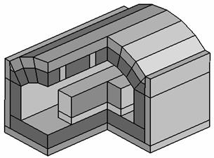
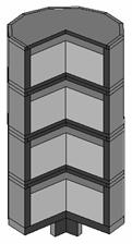
Fig. 3. Geometrical characteristics of numerical models of complex heat transfer

а) Temperature fields of the tunnel oven at different modes of billets heating
b)	c)
temperature fields of the crystallizer growth zone (b), the location and the form of front of crystallization (c)

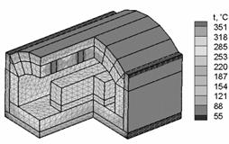
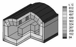
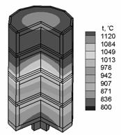
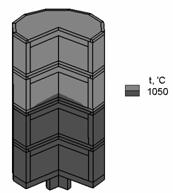
Fig. 4. Results of calculations of temperature fields in conditions of complex heat transfer

Conclusions

A new numerical technique is developed to solve 3D steady-state radiating and radiation-conductive heat transfer problems in conductive and diathermic medium at borders diffusive reflection with accounting of screening effect by direct method of boundary elements.

Research supported by the INTAS Project 05-1000008-8111.

Literature:

1. R.Siegel, J.Howell Thermal Radiation Heat Transfer. – McGraw-Hill Book Company, New York, 1975, 934p.

2. Yuferev V.S., Vasil’ev М.G., Proekt L.B. Novyy metod resheniya zadach perenosa izlucheniem v izluchauzhikh, poglozhauzhikh i rasseivauzhikh sredakh// Jurnal tekhnicheskoy phiziki. – 1997. - Т. 67, N 9. – P.1-7.

3. S.Kochuguev, D.Ofengeim, A.Zhmakin Axisymmetrical radiative heat transfer simulation by Ray Tracing Method, Proceedings of the 3rd European Conference on Numerical Mathematics and Advanced Applications, P. Neittaanmäki, T. Tiihonen and P. Tarvainen (eds.), World Scientific, Singapore, 2000, pp. 579-586.

4. Boundary Element Methods in Heat Transfer/ Ed: L.C. Wrobel, C.A.Brebbia - London & New York: CMP Southampton Boston & Elsevier Applied Science, 1992. - 294 p.

5. C.A.Brebbia, J.C.F.Telles, L.C.Wrobel Boundary element techniquus. – Springer-Verlag, Berlin, New York, Tokyo. – 1984. – 524p.

6. Karvatsky A.Ya., Dudnikov P.I., Leleka S.V., A.I.Juchenko An application of boundary element method to simulate 3D thermal conductive problems //Naukovi visty NTUU “KPI”. –2005.-N5.-P.5-13.

7. Isachenko V.P., Osipova V.А., Sukomel А.S. Teploperedacha /Ucebn. dlya vuzov. - М: Energoizdat, 1981. – 416p.

8. Krasnoshokov Е.А., Sukomel А.S. Zadachnic po teploperedache /Zad. dlya vuzov. - М:Energiya, 1969. – 264p.

9. Phizicheskie velichiny. Spravochnik/ Pod red. I.S. Grigop’eva.- М.: Energoatomizdat, 1991. -1232p.