Comparative analysis of
approximate methods of solving of differential equations for continuously
variable transmissions
Numerous mechanisms based on a pulsed mechanism with unbalanced elements
are available now [1]. Their dynamics is described by systems of nonlinear
differential equations. In general, precise methods of solution for such
equations do not exist. Therefore, in practice, approximate analytical and
numerical methods must be employed. The main analytical methods employ
successive approximation, a small parameter, or power series expansion. Each
approach has its advantages and disadvantages. Therefore, we need to compare
them in order to select the best method for dynamic study of such kind of
transmissions.
A mathematical model of inertia-pulsed transmission may be based on
Lagrangian equations of the second kind. Using this equation, we obtain a
mathematical model of an inertia-pulsed drive in the form of fifth-order system
of non-linear equations
 (1)
(1)
where
![]() is the reduced drag torque on
the driven shaft of the pulsed mechanism,
is the reduced drag torque on
the driven shaft of the pulsed mechanism,
![]() are the moments of inertia of
the elements;
are the moments of inertia of
the elements; ![]() is the total moment of inertia
of the unbalanced elements relative to the geometric center;
is the total moment of inertia
of the unbalanced elements relative to the geometric center; ![]() is the total mass of the
unbalanced elements;
is the total mass of the
unbalanced elements; ![]() is the distance between the
geometric center and the center of mass of the unbalanced elements;
is the distance between the
geometric center and the center of mass of the unbalanced elements; ![]() are parameters of the pulsed
mechanism.
are parameters of the pulsed
mechanism.
To
determine the torque ![]() acting on the driveshaft of the
pulsed mechanism, we use the dynamics characteristic of an asynchronous
electric motor, taking the influence of electromagnetic transient processes
into account
acting on the driveshaft of the
pulsed mechanism, we use the dynamics characteristic of an asynchronous
electric motor, taking the influence of electromagnetic transient processes
into account
![]()
where ![]() is the rated moment of motor
rotor;
is the rated moment of motor
rotor; ![]() are the angular velocity in
ideal idling and the rated angular velocity;
are the angular velocity in
ideal idling and the rated angular velocity; ![]() is the electromagnetic time
constant of the motor;
is the electromagnetic time
constant of the motor; ![]() is the slope of the static
characteristic.
is the slope of the static
characteristic.
For the
sake of comparison, we solve Eq. (1) by several approximate analytical methods.
METHOD OF SMALL PARAMETER
We rewrite Eq. (1)
in the form
 (2)
(2)
where
The
coefficients ![]() contain the moments of inertia
contain the moments of inertia ![]() of the elements of the inertial-pulsed
transmission and are considerably larger than the other coefficients. This
permits the introduction of the small parameter
of the elements of the inertial-pulsed
transmission and are considerably larger than the other coefficients. This
permits the introduction of the small parameter ![]() in Eq. (2). The system then
takes the form
in Eq. (2). The system then
takes the form
 (3)
(3)
On the
basis of the fundamental principle of the method of small parameter, we look
for the solution in serial form
 (4)
(4)
Assuming
that ![]() , we obtain the generating system
, we obtain the generating system
With
the initial conditions ![]() , the solution of the generating system is
, the solution of the generating system is
where ![]()
Retaining
only term where ![]() is of first order and taking
account of the series expansion of the trigonometric functions, we obtain a
system of equations for
is of first order and taking
account of the series expansion of the trigonometric functions, we obtain a
system of equations for ![]()
 (5)
(5)
Solving
Eq. (5) with null initial conditions, we obtain expressions for ![]() and
and ![]()
where
The
solution for ![]() is
is
![]()
where
Retraining only the
first two terms in Eq. (4) and assuming that ![]() , we write the final solution of Eq. (1) by the method of small
parameter
, we write the final solution of Eq. (1) by the method of small
parameter
SUCCESSIVE─APPROXIMATION METHOD
The first
approximation is obtained on the basis of the initial conditions
In
particular, taking account of the first approximation and the conditions ![]() , we obtain the system of differential equations for the second
approximation
, we obtain the system of differential equations for the second
approximation
 (6)
(6)
Solving
Eq. (6) with the specified initial conditions, we obtain the second
approximation of Eq. (1). For the motor torque, the second approximation takes
the form ![]() where
where  .
.
The
second approximation for the angle of drive shaft rotation is
where
The
second approximation for the angle of driven shaft rotation is
where
Confining
our attention to the second approximation for ![]() and
and ![]() , we find the third approximation for the motor torque
, we find the third approximation for the motor torque
 where
where
EXPANSION IN POWER SERIES
By this
method, the solution of Eq. (1) is sought in the form
 (7)
(7)
We find
![]() from the initial conditions
from the initial conditions ![]()
To
determine the second derivatives of ![]() , and
, and ![]() , and the first derivative of
the motor torque when
, and the first derivative of
the motor torque when ![]() , we solve Eq. (1) for higher derivatives
, we solve Eq. (1) for higher derivatives
where
By
differentiating Eq. (1), we find the third derivatives, when ![]()
Substituting the
derivatives in Eq. (7), we obtain the final solution of Eq. (1).
In Fig., we plot
the solutions of Eq. (1) [6], obtained
by approximate analytical methods and by the Runge-Kutta methods.
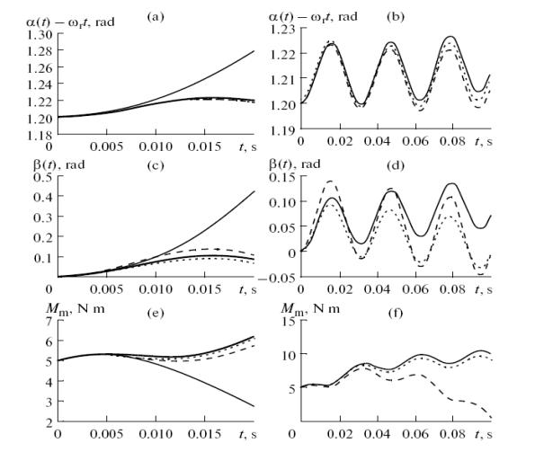
Fig. Dependence of the angles of drive shaft rotation (a, d), and driven
shat rotation (b, e), and motor torque (c, f) on the time t
REFERENCES
1. Leonov A.I.
Inertia-Impulse Automatic Continuously Variable Transmissions, Moscow,
Mashinostroenie, 1978.
2. Alyukov S. V,
Approximate Solution of the Differential Equations of Motion of the Inertial─Pulsed
Transmission. Russian Engineering Research, 2010, Vol. 30, #7.