P.I. Begun, E.A. Lebedeva, D.A. Rubashova, O.V. Shchepilina

Saint Petersburg Electrotechnical University "LETI", St. Petersburg, Russia

BIOMECHANICAL SIMULATION IN MEDICAL PRACTICE

Summary

The questions connected with biomechanical simulation in medical practice are considered. The leading role in biomechanical investigations is played by integral computer method. Considered method is a combination of biomechanical computer simulation and the analysis of biological structures according to the results of clinical (tomography, angiographic, echographic) investigations.

Keywords: biomechanics, simulation, medical practice, finite element package, tomography, angiographic, echographic.

I. Introduction. Introduction into medical practice of new prosthesis methods and assessment of methods of diagnostics is connected with the necessity of enlargement and enrichment of information implementation on wider scale. The absence of necessary information provides objective difficulties and does not allow to plan the success and forecast the result of the operation done technically correctly. In all the basic spheres of the task: medical, technical and fundamental the simulation on the basis of biomechanics of biological object – prosthesis is integral. And the construction of the models of the human body parts functioning in normal state, when pathology and while prosthsesing greatly depends on the use of all the set of new methods and means of investigations. The leading role in biomechanical investigations is played by integral computer method. This method is a combination of biomechanical computer simulation and the analysis of biological structures according to the results of clinical (tomography, angiographic, echographic) investigations. The complexity of geometrical shapes of investigated biological objects, their inhomogeneity and anisotropy of their structural mechanical properties predetermined the construction of mathematical models in the frames of three-dimensional body mechanics and parametric models built in finite element package Solid Works, Cosmos Works, NASTRAN, COMSOL, ANSYS. Interactive software package Mimics allows to visualize and segment the images received with the help of tomography and construct biological objects on the base of tomography.

II. Problem definition. The simulation process consists of the allocation of object’s properties and its interaction with other objects, the notification of the peculiarities in functioning in different external influences and logic analysis of the information received. The model is a speculative idea of a real object which reflects the characteristics of the real object which are necessary to get an answer to the given task.

The usage of computer programs based on numerical methods allows to delve into the fields which cannot be served by analytical methods due to large complications in implementation. Analytical approach and the computer numerical method are interpenetrative and supplemental each other methods. With powerful software numerical computer analysis takes up dominant position.

Physical modeling is based on reproduction of biotechnical objects, functions and processes with physical methods. Physical modeling allows to replace investigation of a real object by the research of characteristics of reduced or increased mechanically similar model with the following transition from the model parameters to the corresponding parameters of biotechnical object. The scientific base of physical modeling is the similarity theory. The methods of similarity theory allow to transfer from reference physical values to some generalized variables – similarity criterion. This allows to decrease the quantity of physical parameters describing the phenomena and get a large alliance of the received result.

Modeling process consists of allocation of characteristics of the object and its interaction with other objects, reflection of peculiarities in functioning at different external influences and logic analyses of gathered information.

The model reflects the structure and function of the original system by means of structure and functions of those elements it is built of.

III. Results. We will illustrate told above on examples.

Example A. Modern problems of rehabilitation after hip fracture due to the fact that is not governed by the maximum load, taking into account the recovery of bone regenerate and is not considered a risk of vascular disorders. At the same time during postoperative period after the hip fracture results from the fact that the thighbone traumatic injury affects the locomotor system kinematic reactions in general, thus facilitating associated disorders that do not directly result from the injury, yet worsening the patient’s life.

Despite new implant designs, improved skills of surgeons, new operation methods implemented, the results stop satisfying patients as the full recovery period reaches half a year. This is because the missing is the individual approach depending on the bone tissue condition, the fracture location. The issue of the bone graft reconstruction at the subcapital fracture location lacks attention.

However, information technologies development in medicine, particularly in trauma surgery, orthopedics and biomechanics allows achieving radically new rehabilitation technology level.

The object of the research is to develop thighbone diagnostic technique after osteosynthesis with muscle activity and elasticity module (E, MPa) taken into account at every bone graft remodeling stage. The algorithm has been developed, the calculations have been carried out and the analysis and the research have been undertaken for the “thighbone-bone graft-implant” system stress and stain behavior at various rehabilitation stages.

The following assumptions were considered while building the conceptual model:

1) thighbone bone structure is idealized to comprise two isotropic layers: cortical and spongy;

2) within the thighbone, the fissure is located at the thighbone neck cross-section and it has uniform isotropic structure, wherein its mechanical properties change at every osteotylus reconstruction stage and those are localized within the zone that is free of muscular efforts;

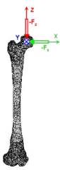
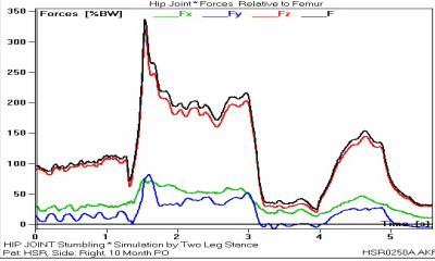
3) dynamic stress is applied to the thighbone center by axes X, Y, Z (www.orthoload.com).

Figure 1 represents experimental data, with the coordinate system selected axes orientation and coordinate center within the thighbone shown (a), as well as the example of the effective load changes as a function of time (b).

a	b
Fig.1. Test data

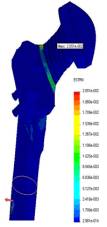
As initial data, the thighbone MRT is used to build the object 3d models by means of Mimics, the computer modeling environment. With those models imported into the Solid Works software package, a solid thighbone geometric model was obtained with damages at the area of the greater trochanter. The considered is the bone recovery via osteosynthesis, with two cannulated titanium screws.

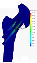
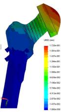
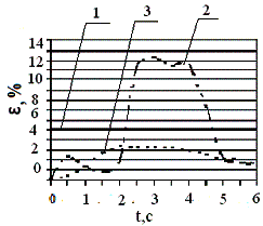
In terms of non-linear dynamic analysis, various rehabilitation procedures, relating to the first two rehabilitation stages, were considered. The obtained results are represented via fig.2. Figure 2 represents the stress diagram (a), displacement (b), deformations (c) to the femur at the hip abduction in the side in a sitting position and represents dependences of deformations appearing at the first stage with E_per=5.4kPa ( d): 1 – allowed deformation, 2 – deformation with the thigh aside, 3 – deformation for the thigh up 30°.

a	b	c	d
Fig.2. The first stage of rehabilitation

The following was concluded there from:

1) the tendency was discovered of the deformation depending on the elasticity module E, thus this factor must be taken into consideration when developing rehabilitation programs, particularly for the initial stages of the rehabilitation, when the bone structure has not fully restored after the damage yet, and the blood vessels are vulnerable for significant deformations;

2) putting a thigh aside during the first stage of rehabilitation, as well as walking with support on the bad leg are counter-indicative for patients with the subcapital fracture who underwent osteosynthesis.

Example B. There are several methods for measuring intraocular pressure. The Maklakov’s method is the most common in Russia. The method of determining intraocular pressure by Maklakov’s tonometer is based on installing a particular weight with a flat surface on the eye. Under load, the surface of the eyeball flattened by tonometer’s contact surface to a certain flattening circle. The value of the tonometric intraocular pressure is determined according to the diameter of the flattening circle of corneal by the contact part of the tonometer. To converse the tonometer readings to pressure in the unit mm Hg. Art. special calibration tables or straightedges are required. Internals of the eyeball’s structures are not taken into account while measuring of intraocular pressure. Numerous studies in the field of ophthalmology has shown that the variability of the thickness and curvature of the cornea significantly affect the results of tonometry. But, the influence of keratoconus on the measurement’s results has not been considered yet. The corneal curvature radius and the thickness of the central zone changes with keratoconus. Ultimately it becomes thinner and takes a conical shape (Fig. 3).

Fig. 3. The scheme of the model of the eye with the connective tissue formations orbit

There are three stages of keratoconus: at the first stage of keratoconus there are reduction of visual acuity, decrease in the radius of curvature of the cornea to 7.5-7.2 mm, decrease of the thickness of the central corneal zone to 0.48 mm; at the second stage of the disease the deformation of the cornea progresses, the radius of curvature decreases to 7,1-6,75 mm, the thickness of the central zone of the corneal - to 0.44 mm; at the third stage the cornea becomes thinner, and its radius decreases to 6,7-6,0 mm, the thickness of the central corneal zone - to 0.40 mm.

To investigate tonometric IOP in normal and keratoconus development model was built based on the eye orbit connective tissue formations (Fig. 3). Tonometric IOP was calculated sequence of iterations as a result of which the volume is not the flattened area of the deformed eye includes an additional amount of fluid displaced from corneal tonometer:

1. Defined volumes: a) deformed eyes, b) aqueous humor displaced tonometer flattened part of the eyeball, in) is not the flattened area of the deformed eyeball;

2. Conditions of zero displacement in the cornea, in the contact zone with the tonometer, calculated displacement and deformation is not flattened cornea and sclera;

3. Assuming a linear relationship between load and displacement, as defined in claim 2 nonoblate character deformation of the eye , increased its volume by 0.9 volume of fluid displaced by the tonometer;

4. Similarly, paragraph 2 provides the equilibrium condition in the contact zone of the deformed cornea and the tonometer;

5. Defines the scope of the non-flatness of the eyeball;

6. If the volume is not different from the flattened part of the original volume of the eyeball, amended in accordance with paragraph 3 (increases or decreases the volume of the eye is not flattened;

7. If necessary, consistently repeated the calculations in accordance with § 4-6.in accordance with р. 4-6.

Research of keratoconus’s influence on the parameters of intraocular pressure is held with applanation load of 10 g and with the diameter of the flattening circles are 3, 4, 5, 6 and 7 mm. Compliance of the diameter of the flattening circle and the tonometric pressure P_М is established according to B.L. Polyak’s rule.The geometric constructions of the models were developed by the Solid Works computer program. Stress-strain condition was calculated by Cosmos Works finite-element software.

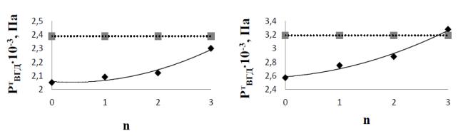
Fig. 4 shows the calculation results of tonometric intraocular pressure for the model at three stages of keratoconus (n = 1, 2, 3).

a	b
Fig. 4. The dependence of the investigated tonometric intraocular pressure (slanting line) and intraocular pressure detected by the Maklakov’s method in accordance with the rule of B.L. Polyak (horizontal line) from the stage of keratoconus calculated according to the model, flattening circle diameter of 7 mm (a) and 6 mm (b).

In the study of the influence of keratoconus on tonometry results introduced the following sumptions: 1) the material of the cornea, sclera, dura mater, tennonov’s capsules, fasciae musculares materials, episcleral space and orbital bones is uniform, solid and isotropic with reduced modulus of resilience; 2) the model is rigidly fixed on the outer side of the eye socket bone; 3) modulus of resilience of the cornea E_P = 0.362 MPa, modulus of resilience the contact part of the tonometer E_T = 210 GPa; reduced modulus of sclera, dura mater, tennonov’s capsules, resilience fasciae musculares, episcleral space and orbital bones are equal respectively E_C = 6 MPa; E_TMO = 150 MPa; E_ТК = 200 MPa; E_CT = 20 MPa, E_Э= 30 kPa, E_К = 2.5 GPa. 4) the radius of curvature of the cornea in a normal state (n = 0) R_КР = 7.8 mm, the central zone thickness h_РЦ = 0,52 mm, thickness at the periphery of the cornea assumed to be constant at all stages of keratoconus h_РП = 0.6 mm. At the next three stages (n = 1, 2, 3) cornea changes its curvature R_КР = 7.2 mm (n = 1), 6.8 mm (n = 2) and 6.2 mm (n = 3) and central zone thickness, respectively h_РЦ = 0.48 mm, 0.44 mm and 0.4 mm; thickness and radius of curvature of the sclera H_C = 0.7 mm R_KC = 12 mm, diameter dura mater D_H = 2.1 mm; the thickness and radius of curvature tennonov’s capsule H_TK = 0.74 mm, R_TK = 13 mm; dimensions fasciae musculares T_СТ = 5 mm, t_СT1 = 11.25 mm, t_СT2 = 16 mm, h_СT1 = 0.7 mm, h_СT2 = 1.76 mm, outer diameter fasciae musculares d_СT = 36.7 mm, height of the orbit Н_Г = 52.5 mm outer diameter orbit D_Г = 49 mm, inner diameter of the orbit d_Г = 33 mm.

The model is divided into 70000 tetrahedral finite elements. With the increasing of the stage of keratoconus development Corneal of the eye becomes more pliable. When flattening circles are from 7 mm to 3 mm, intraocular tonometric pressure increases relative to the norm from 10, 8% to 37.3%. With the increasing of the stage of keratoconus's development the discrepancy of calculated tonometric intraocular pressure and tonometric intraocular pressure detected by the Maklakov’s method decreases.