Gudukhina А.A., Chernysheva L.P., Yasinskiy I.F., Koltsova E.A.
Ivanovo State Power
Engineering University
Ivanovo, Russia
Simulation of fluid
flow in systems with different internal configuration using parallel
technologies
I.
Introduction
Hydrodynamics
is a section of the aerohydrodynamic science, which studies the motion of
incompressible fluids and their interaction with solids. Compressibility means
the ability of a substance to change its volume under the action of
comprehensive pressure.
The objectives
of this paper:
· creation
of an application for modelling hydrodynamic systems
· exploration
of possibilities to accelerate computations using parallel programming
technologies
· comparison
of the results of the gradual and parallel implementations
II.
Mathematical model
A. Basic
hydrodynamic equations
Navier-Stokes and continuity equations are used for modelling
hydrodynamic systems in this research, as the mathematical model is the most
popular among similar scientific papers. That means that fluid is ideal and its
volume will be the same during the whole process of modelling. The system of
equations (1) describes fluid flow in two-dimensional coordinates.
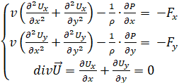 (1)
(1)
v – kinematic
viscosity coefficient, P – pressure, r - environment
solidity, ![]() – velocity.
– velocity.
B. The
algorithm for solving the hydrodynamics problem
1. Initialization of velocity and pressure fields.
2. Calculation of a new pressure field using old
velocity field.
3. Calculation of a new velocity field using new
pressure field according to system (1).
4. Recalculation of boundaries.
5. If one more step is required, go to point 2,
otherwise stop calculations.
C. Boundary
and initial conditions
Two types of boundary conditions are used in
this system. The first one is solid boundary. Speed axis rates are equal to
zero here. Supply and exhaust vents have one speed axis rate equal to zero, and
the other one is calculated in the way to get parabolic profile: numbers near
boundaries are seeking a null position and the maximum value is in the center
of a vent. Initially, the velocity and pressure fields in the entire modelling
area are determined to be zero. The speed is set only on supply and exhaust
vents.
III. Investigation
of systems with diffeent internal configurations
Using the system of equations (1) and described boundary and initial
conditions, systems with supply and exhaust vents were composed.
Figures 1 and
2 show stable hydrodynamic systems where arrows indicate the direction of fluid
movement in the system, and their length schematically indicate the velocity of
the fluid: the shorter the arrow, the slower the speed. The brightness of cells
indicates the degree of pressure at a certain point in the system.


Figure
1 Figure
2
By simulating the process of fluid flow in a confined
space, we can determine in advance whether a system is stable and how it could
be stabilized. Considering pressure in a system will show the places which are
the most vulnerable to the impact of flow.
IV. Parallel algorithm
CUDA technology gives an opportunity to parallelize calculations on a
grid of processors. Every processor can calculate one or several values on
every iteration. Obviously, this approach will be more beneficial for us.
Instead of calculating values in each point one by one, each thread chooses a
task according to its coordinates and calculates three values for each point.
Table 1 contains time (in seconds) of gradual and
CUDA algorithm realizations work.
Table 1 – Time of algorithms
work
|
System
Order |
100 |
300 |
500 |
700 |
900 |
1000 |
|
Gradual |
7,6 |
109,9 |
280,5 |
548,7 |
852,9 |
904,9 |
|
CUDA |
1 |
7,68 |
20,95 |
40,64 |
66,57 |
82,07 |
According to numbers presented in
table 1, CUDA algorithm is ten times faster than the gradual one.
V. Conclusion
Modelling of hydrodynamic systems is a scientific
sphere, which allows carrying out experiments and not exposing real systems to
danger. Visualization of a fluid flow and pressure distribution makes
calculations spectacular for scientists.
Mathematical model described in the paper provides
opportunity to model fluid flow in constraint environment and its parallel implementation
allows getting calculation results faster. The next step in this project will
be the creation and implementation of parallel algorithms with different
technologies.
References
1. Filatov E.I., Jasinski F.N., Matematicheskoe
modelirovanie techenij zhidkostej i gazov: ucheb. posobie Ivanovo: ISPU, 2007,
84 pp.