Kapchenko
M.M.
Simulation of an empirical relationship between Dow Jones
Industrial Average and S&P 500 index
Consider the sampling with the value of
the index S&P 500 and Dow Jones Industrial Average. The values were
recorded every minute during the auction.
Here are some theoretical reference:
The
S&P 500 (Standard &
Poor's 500), is an American stock market index based on the market
capitalizations of 500 large companies having the largest capitalization. Dow Jones Industrial Average is
a stock market index created by Wall Street Journal editor and Dow Jones &
Company co-founder Charles Dow. This index was created to monitor the
development of the industrial component of the US stock markets. For its
calculation used the average scalable - the amount of the price is divided by
the divisor, which changes whenever stocks included in the index is subject to
fragmentation (split) or association (consolidation).
Let's
identify the relationship between them.
At
the beginning consider the matrix scatterplot(Var1-SP, Var2-DJ):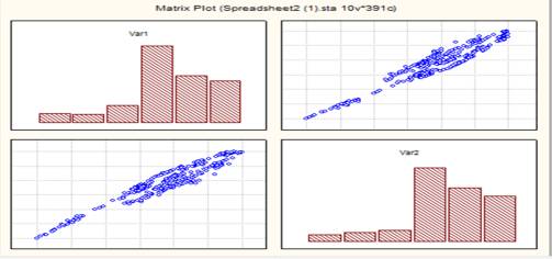
As we can see in the diagram there is a clear relationship between these
indices. To check it, let's conduct the corresponding regression:
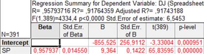
Thus,
the model has a rather high coefficient of determination ![]() = 0.91743188
= 0.91743188
Model addiction, adjusted by the
method of least squares is:
DJ ≈ -855.525 + 9.364*SP
Let’s do analysis of residues:
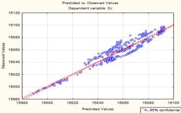
The scatter plot Predicted - Observed values shows that the prediction formula captures the basic trend observations.
Now Consider the scatter plot Predicted - Residual scores: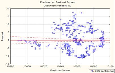
On diagram clear dependence are not
observed. The points are scattered randomly, indicating the inability to
improve the prognosis of the available data. Let's verify the normality of the distribution of errors.
To do this, we
construct the diagram quantile against quantile (Q–Q plot):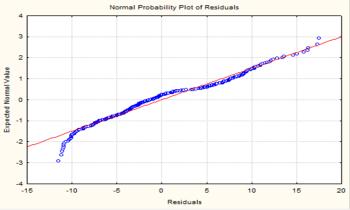
We can see that errors follow a
normal distribution.
Now let's construct confidence
intervals for the regression coefficients. For this we use the following
formula:
![]()
N = 391, we believe that α =
0,05 then using a probability calculator we have:
![]() =
1,967930
=
1,967930
![]() -855.525 тоді
-855.525 тоді ![]() = -855.525 ± 1,967930 * 256.9112
= -855.525 ± 1,967930 * 256.9112
![]() [-1361.1082; -349.9417]
[-1361.1082; -349.9417]
![]() 9.364 тоді
9.364 тоді ![]() = 9.364 ± 1.967930 * 0.1422
= 9.364 ± 1.967930 * 0.1422
![]() [9.0842; 9.6438]
[9.0842; 9.6438]
Thus, we have obtained a regression
model DJ ≈ -855,525 + 9,364*SP
with a relatively high coefficient of determination, which can be applied in
practice to calculate the Dow Jones Industrial Average through the S&P 500 index.
References
1. KARTASHOV M.
Probability, Process, Statistics. Publishing and
Printing Center Kyiv University' 2008.
2. Majboroda R.
Regression: linear models. TViMS,
2004 - 283 p.
3. Leonenko N., Tinsel Y., Parkhomenko V. and Yadrenko M.
Theoretical-probability and stochastic methods in financial mathematics and
econometrics. K .: Informtehnika, 1995. - 380 p.