Экономические науки/ 8.Математические методы в экономике.

К.т.н., Полинский А.М.

Студент Загорулько К.А.

ГВУЗ «Национальный горный университет», Украина

Monte Carlo Simulation and its Use in Everyday Business

If you were to flip a coin 100 times, you’d expect to end up with about 50 heads and 50 tails. This is common sense and very simple probability; however, it is also the basic principle of Monte Carlo Simulation. Things get interesting when you have a process where either or both of the below are true:

· There are multiple steps and options where basic logic/calculations cannot easily determine the expected outcome.

· The possible outcome does not appear to follow any obvious pattern or predictable outcome.

To further explain this theory, imagine a typical process such as an employee driving to work – for this example we will ignore any associated cost difference, and instead focus purely on time:

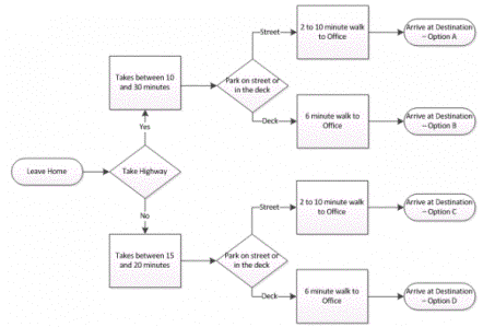
On any given day the employee in the process above can choose between four different paths to get to his or her destination. In some rare processes the distribution for the time ranges (e.g. ‘between 10 and 30 minutes’) may be known, for example in a factory where employee X can assemble a widget in 10 minutes, and employee Y assembles the same widget in 30 minutes. However, in most scenarios – and where Monte Carlo really shows its value – is when the distribution is unknown and continuous.

In the example, I provided a range of how long it took the employee to get to work using the highway. Imagine now that for a period the actual time for each decision was recorded and rounded to the nearest minute. With this data it is possible to create a probability mass function or ‘PMF’ (# of occurrences that it took the specified amount of time/total attempts). The x axis represents the time taken rounded to the nearest minute, and the y axis represents the PMF.

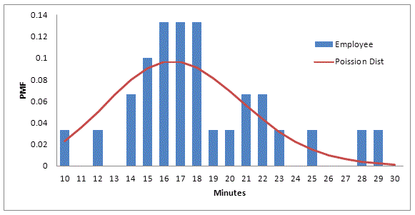
Using your PMF and some statistics software (e.g. @risk), you can estimate the distribution that matches your data. In the example above the data appears to loosely fit a Poisson distribution with a mean of 17 (overlaid in the red).

After you have calculated all of the distributions for the unknown functions within your process (for the example above it would be 3, with one used twice), it is time to begin the fun part of Monte Carlo Simulation.

For each distribution, run a simulation a number of times (usually a minimum of 100) to calculate the mean and any other statistics that might be useful (e.g. standard deviation) for your process. Using your new found values, calculate the expected outcome for each of your end scenarios. In our example, this translates to whether the employee should use the highway or not, and whether he or she should park on the street.

The example provided above is an overly simplified use of Monte Carlo, and the exact steps vary depending on the software suite you plan to use. More often than not, a tool will allow you to map out the process/distributions and then run the simulation all together, so rather than calculating each of the distributions separately, it will simply show you the results of all of the final outcomes. What is great about Monte Carlo is it allows you to use extremely complicated distributions based on actual data, rather than just using a mean or basic probability function. Furthermore, knowing standard deviations and how well the selected distribution ‘fits’ the data allows you to provide very accurate confidence intervals around how good the model. Furthermore the models can also produce probability for exceeding or beating a targeted number (e.g. what is chance the trip takes over 25 min).

Monte Carlo analysis can be used for much more than just process assessment and design. For example, consider a large system change where projects are underway to replace an old system that interacts with lots of users. Process engineers can help by leveraging Monte Carlo analysis in the following ways:

· Organizational Change Management – by using a sample group of participants, you could estimate costs and time involved in migrating users to a new business system. This approach may also help identify trouble areas and where additional resources may be required.

· Testing – using previous testing data for the corporation, it is possible to provide estimates around the predicted max and minimum amount of time required to test a known amount of test sets and hence a number of testers needed.

· Project Management – by considering the areas above (and more), Monte Carlo could accurately provide the likely outcome of the whole project schedule and costs based on known variances and historic results for the company.

There are many more examples that could be listed here, and this is just the tip of the iceberg of uses for Monte Carlo. Feel free to contact me with other ideas in which Monte Carlo analysis could apply, and especially to ask any questions on how specifically to apply Monte Carlo to any process problems you may be facing.

Links:

1. Berkowitz, J., O’Brien, J., 2002. How accurate are the value-at-risk models at commercial banks? J. Finance 57, 1093–1112.

2. Corradi, V., Swanson, N., 2006. Predictive density evaluation. In: Elliot, G., Gringer, C., Timmcrmann, A. (Eds.), Handbook of Economic Forecasting. Elsevier, North Holland, vol. 1. pp. 197–284.

3. Crnkovic, C., Drachman, J., 1996. Quality control. Risk September 9, 138–143.

4. Gaglianone,W., Lima, L., Linton, O., 2011. Evaluating value-at-risk models via quantile regression. J. Bus. Econ. Stat. 29, 150–160.