ON BICRITERIAL OPTIMIZATION OF WELL-DRILLING SELF-COST

Економічні науки / Економіка підприємства

УДК 681.513.54

Fadyeyeva I.G.

Ivano-Frankivsk national technical university of oil and gaz

ON BICRITERIAL OPTIMIZATION OF WELL-DRILLING

SELF-COST

It is known [1,2], that one of the most general and universal criterion of well-drilling process optimization is the minimum of cost-price of 1m of drilling. Statistics [2] testifies, that now for the drilling of one deep borehole (over 4000m) the USA use 19 bits, European countries use 60 bits, in the countries of the former Soviet Union (Ukraine includea use about 300 bits).

The analysis of results of well-drilling in Ukraine demonstrates [4], that more than 50% of emergencies in wells are the result of wrong exploitation of drilling tool. Monitoring a technical condition of drilling tools and shorts term forecasting of well drilling cost is an important task, which defines the efficiency of drilling process [3]. Consequently, development of more general and universal criterion of well-drilling process optimization is of great interest .

Formulation of the problem. Drilling of a borehole includes the choice of equipment, drilling method, geometrical size of the well, type of chisel, quality and quantity of the washing liquid and technological parameters, such as axel loading on chisel and its rotation speed. There is also a demand for organization of drop-and-lifting operations forecasting of emergency and completition of the well.

Problems of well-drilling optimal control could be devided into problems which are to be solved at the optimal project planning stage and those ones to be solved during the well-drilling process. The second group of problems is most difficult and important, since the efficiency of drilling enterprise’s activity much depends on them. As numerous investigations show, succesful handling of these problems make it possible to decrease well-drilling costs by 25-30%. At the same time the development of the new drilling technique does not significantly influence the decreasing of costs.

Adaptation of technological parameters, quality and quantity of the washing liquid and chisel’s type can be performed in accordance with fhe chosen optimality criterion. In general case these criteria are devided into economical, technical and technological, and informational ones. The economical criteria are the more preferable for deep oil and gas well-drilling, because the costs-prise is one of the deciding indicators of this process.

The most important economical criterion is the well-drilling cost-prise B_c. It includes material expences, expences for chisels, pipes, usage of equipment and organizational and technological elements, as well [2].

Cost-price B_c essentially depends on the well-drilling time T end borehole depth H. So, the optimization problem sounds

, (1)

where x=(T, H) and S is the feasible region (H may be divided into N stages).

The most important technological criterion is the drilling time T leading to the following task

, (2)

with x and S as above.

From a technological point of view T can be divided into three components at i-th drilling stage, namely drilling time t_δi, drop-and-lifting operations time t_cni and auxiliary operations time t_bi (including replacement of chisel, waching of the borehole, and other control and supporting activies). Hence, we get

. (3)

The drop-and-lifting time t_cni is defined as

, (4)

where H_i is the depth of the borehole at the end of ith stage; v_i is the average speed of drop-and-lifting.

Because , where h_k is the width of stage and then we get from (4)

. (5)

Up to now, the well-drilling process is optimized by choosing costs or time as objective function imposing restrictions or the other indicator. Often, the cost-price B_c is preferred, because it takes into account not only technical indices, but economical ones, as well. However, the “one-criterial” approach is not always most suited, because it may lead to loss of information or it even may hide desirable compromiss solutions. Thus, we are led to multicriterial optimization tasks. This also illustrated by Fig.1 where for sake of completeness the whole algorithm of well-drilling optimization is given.

As one can see, there are three control levels in the drilling process (indicated by roman numerals). Problems of well-drilling control at technological level I (chisel’s trip) is solved as bicriterial crisp optimization with objective functions B_c (min) and speed of chisel’s trip V_p (max). At stage III we are faced with the performance criteria profit PR (max), costs of well-drilling B_cb (min) and well-drilling time T_pr (min). The problem under consideration is settled at stage II, namely drilling of the borehole till projected depth.

As already mentioned we are faced with the following bicriterial optimization task

. (6)

The feasible region S is given by

(7)

In Section III we discuss some details concerning this kind of optimization. For basic notions, theorems and methods we refer to [5].

Fig.1 Algorithm of well-drilling multicriterial optimization

Results. We tooke for investigation 3 models: retrospective model, crisp operative model and fuzzy operative model.

Retrospective model. The criteria are based on retrospective analysis of experimental data gathered from borehole SPAS-101 located in the Carpathians in the Ukraine at a depth of 4160-4510 meters. For efficient operative control information is gathered daily what will result in a virtual segmentation of the borehole interval (of width H=450 meters) in N layers of width h_i; i=1,…, N. Hence, we have

, (8)

with T_i = t_δi + t_cni + t_bi in accordance with (3). Here, we have N=45. Drilling time t_δi is given by such meaning:

. (9)

The auxiliary operations time is constant: t_bi = 1 hour. The other quantities in (9) are as following (i = 1,…,45): relative wearout of the chisel =0,02+(i-1)·0,022 [1/h]; initial drilling speed [m/h] (see Table 1): drop-and-lifting speed v_i=250 [m/h].

Table 1.

i	1	2	3	4	5	6	7	8	9	10	11	12
	0.75	1.154	1.333	1.714	1.2	1.074	1.5	0.923	1.333	2	1.714	2.4

13	14	15	16	17	18	19	20	21	22	23	24	25	26
4.285	4	1.5	1.09	1.2	1.714	1.2	1.714	1.764	2.22	2	2.5	1.714	1.25

27	28	29	30	31	32	33	34	35	36	37	38	39	40
2	1.333	2.4	2	1.875	1.333	2	1.714	1.333	1.5	1.333	0.857	1.5	2

41	42	43	44	45
1.741	1.2	2.4	1.714	1.578

Criterion B_c is given by mean specific costs as

(10)

with the next meaning i B_ci

(11)

with T_i as in (8).

Here, we have :

specific cost of drilling unit work B_o=82 [1/h];

cost of the chisel B_g=6425.4 [units].

(During the optimization we omitted the constant factor ).

Crisp operative model. In opposite to the above model we now consider models permitting operative control. This means that we are able to control the process by the axial loading on the chisel P_i and rotation speed n_iin each segmentation i. It turns out that the above introduced values h_i, T and B_c depend on these technological parameters. Here, N=15 proved to be sufficient for modelling the process.

Again, (8)–(9) is valid with

. (12)

The overall costs are given by

, (13)

where the costs of segment i reads as

(14)

with

. (15)

Here [3],

. (16)

Coefficients k, k_j, α, α_j ,β, β_j (j=1,2) depend on the geological properties and are a result from regression analysis. Their numerical values are listed up in Table 2.

Table 2.

k	k₁	k₂	α	α₁	α₂	β	β₁	β₂
0.006	25	1	0.4	0.05	0.15	0.25	0.1	0.15

The are the same as in Table 1, but only every third value is accounted. The feasible set S now reads as

. (17)

Fuzzy operative model. In reality, however, drilling conditions (physical and mechanical properties of rocks and chisel, washing liquid and drilling column properties) may change, thus leading to parameter uncertainties. The latter may have dynamic, stochastic and/or nonstochastic character [3]. To estimate the latter, often experts statements are available. Here, we are faced with the typical situation that the specific costs B_cifor ith segment are given as a rule-based system with nonstochastic uncertainties, namely

if T_i is and h_pi is then B_ci is ; j = 1,…, M. (18)

Here, (k = 1,2,3) is a linguistic expression like “small”, “medium”, “big”, etc., whereas M means the number of rules. The complete rule base is given in the following matrix (where indeces “i” are omitted for simplicity).

h_p T	VS	S	M	B	VB
VS	VB	B	VS	VS	VS
S	VB	B	S	S	VS
M	VB	B	M	S	VS
B	VB	B	B	S	S
VB	VB	VB	B	B	B

VS – “very small”, S – “small”, M – “medium”, B – “big”, VB – “ very big ”.

Since fuzzy sets theory has proved to be a powerful tool for modeling such kind of uncertainties and statements, we decided to model the linguistic expressions by fuzzy sets. The rule base is tackeled as Takagi-Sugeno system. Though the current inputs are crisp (real numbers) the result will be fuzzy due to the fuzziness of the outputs. Hence, we applied a defuzzification procedure to get numerical outputs [3].

Denoting the fuzzy sets (and somehow loosely speaking their membership functions, as well) in the jth rule by and we obtain for current crisp inputs the corresponding input evaluation as

, (19)

where t means a suited triangular norm (we took the product).

The current output will be obtained (applying fuzzy arithmetic) as weighted mean over all rule output, i.e.

, (20)

where the denominator is assumed to be positive.

It is well-known that is a fuzzy number as well. For optimization we need, however, a crisp output, that is we have to defuzzify . The level sets of any fuzzy number are closed intervals on the real axis [4,6,7]. Denote them by for we can defuzzify by suited integral means, e.g.

, (21)

where the existence of the Rieman integral in (21) is ensured by the monotonicity of .

Hence, now our model for the overall costs becomes

(22)

with use of (19)-(20).

Results of optimization. All three models were investigated w.r.t. their bicriterial Pareto optims whereby the compromise function was used. As optimization method we applied Powell’s Direction Set Method [8], which is fairly efficient without using derivatives. Restriction (7) was taken into account as penalty.

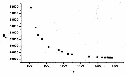
Retrospective model. First we took α uniformly distributed as shown in Fig.2

Fig.2 Pareto set for the Retrospective model (uniformly distr. α)

One sees that for T >1200 there is an undesired accumulation of points. That is why the Pareto curve was approximated by the following rational function [4]

with the coefficients

a =17427,85; b = -7232071,5; c = -4207299e+9; d = 0,37878;

e = -147,213; f = -106855,6.

The corresponding α were determined and we obtained the following Pareto set:

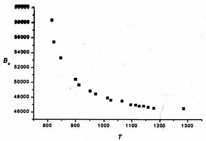
One realizes that the distribution is improved (far from being ideal). The corresponding Pareto points are listed up in the below table (for shortage of space we do not itemize the 45-dimensional solution vectors).

Fig.3 Pareto set for the model

Table 2.

i	1	2	3	4	5	6	7	8	9
T	814	822	847	900	912	951	971	1013	1025
*B_c*	58316	55432	53283	50393	49644	48819	48436	47905	47590

i	10	11	12	13	14	15	16	17
T	1065	1096	1114	1127	1142	1159	1179	1186
*B_c*	47464	46985	46935	46800	46796	46647	46511	46470

From the decison-makers viewpoint most interesting seem to by points 4 ands 5, because they indicate some break: onthe left-hand side we gain a lot for B_c with only small losses w.r.t. T. Right from these points the gain for B_c becomes rather small while we have to note a greater loss of T.

Crisp operative model. Here we had to allow with more numerical difficulties due to the high nonlinearity of the functions involved. Hence, a smaller number of Pareto solutions was obtained .

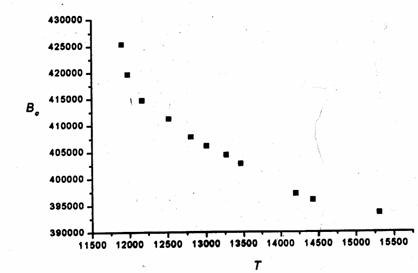
The corresponding data are contained in the following table (again the solution vector of dimension 30 is omitted).

Fig. 4 Pareto set for the crisp operative mode

Table 3.

i	1	2	3	4	5	6	7
T	11907	11986	12173	12522	12807	13010	13272
*B_c*	425376	419672	414701	411259	407867	406148	404424

i	8	9	10	11
T	13468	14206	14429	15311
*B_c*	402774	397144	395988	393535

Obviously, the neighbourhood of point 3 seems to be worth being investigated further.

Fuzzy operative model. The situation is analogical to the previous one.

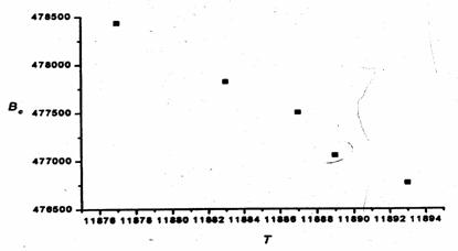
Fig. 5 Pareto set for the fuzzy operative model

Notice, anyhow, that the evaluated set of drilling time T is narrowed in comparison with the crisp model what is due to the information submitted by the experts.

Table 4.

i	1	2	3	4	5
T	11877	11883	11887	11889	11893
*B_c*	478435	477821	477503	477054	476767

Here, point 4 is most interesting from the decision makers view point.

Summary. In opposite to the classical approach of decision making in well-drilling that is based on objective function, the method presented here enable to exploit the derived models in a more efficient way w.r.t. finding “good solution”, i.e. preferable parameters for controlling the process. With the help of the Pareto set one is able to determine compromisses which are more satisfactory from user’s point of view because the behaviour of drilling time and costs (w.r.t. optimality) can be taken into account simultaneously, The fuzzy model, however, turns out to be too coarse for final decision making. Hence, a finer and more sophisticated partition of the time and segmentation universums and the costs, as well, seems to be advisable to get a more sensitive response function.

References

1. Maric V.B., Criganivsciy E.I., Dovgoc V.E., Gouc R.Y. Actual problem of roll-bit. Exploration and development of oil and gas deposits.–2003.–V. №2(7) .– P.109-113.

2. Furness R., Wu C., Ulsoy A. Statistical analysis of the effect of feed, speed and wear on hole quality in drilling. I Manufect SciEng ,1996.– P.367-375.

3. Chygur I, Fadyeyeva I, Sementsov G.. Application of fuzzy logic for the simulation of drilling tools wear process and short-term forecasting of well-drilling cost. Proc.10^th Zittau Fuzzy Colloquium, Sept.4-6, 2002.–P. 173-177.

4. Das I., Dennis J.E. A closer look at drawbacks of minimizing weighted sums of objectives for Pareto set generation in multicriteria optimization problems. Price Univ., Houston, Texas. Working Paper, 1996.–12 p.

5. Ester J.. Systems Analysis and Multicriterial Decision Making (in German) VEB Verlag Technik, Berlin, 1987.

6. Eschenamer H., Koki I. and Osyczka A.. Multicriteria Desing Optimization. Berlin, Springer-Verlag, 1990.

7. Koski I.. Multicriteria Truss Optimization. Multicriteria Optimization in Engineering and in the Sciences. Edited by Staler W.. New York, Plenum Press, 1988.– P.175-179.

8. Press W.H. et al., Numerical Recipes in Cambridge C. Univ.Press, Cambridge, 1988.