Tехнические науки/ Авиация и космонавтика

Nickolay Zosimovych

Instituto Tecnólogico de Monterrey (Campus Gualajara, Mexico)

INTEGRATED GUIDANCE SYSTEM OF A COMMERCIAL LAUNCH VEHICLE

In the article has been chosen and modeled the design objectives for an integrated guidance system of a commercial launch vehicle with application of GPS technologies. Was set the conceptual design of an integrated navigation system for the space launch vehicle qualified to inject small artificial Earth satellites into low and medium circular orbits. The conceptual design of the integrated navigation system based on GPS technology involves determination of its structure, models and algorithms, providing the required accuracy and reliability in injecting payloads with due regard to restrictions on weight and dimensions of the system.

Keywords: Gimbaled inertial navigation system (GINS), global positioning system (GPS), inertial navigation system (INS), mathematical model (MM), navigation, pseudorange, pseudovelocity, launch vehicle, self-guided system (SGS), Kalman filter, control loop, control system (CS), trajectory, boost phase (BPH), distributor, coordinate, orientation.

Introduction. A key tendency in the development of affordable modern navigation systems is displayed by the use of integrated GPS/INS navigation systems consisting of a gimbaled inertial navigation system (GINS) and a multichannel GPS receiver [1]. The investigations show [2, 3], that such systems of navigation sensors with their relatively low cost are able to provide the required accuracy of navigation for a wide class of highly maneuverable objects, such as airplanes, helicopters, airborne precision-guided weapons, spacecraft, launch vehicles and recoverable orbital carriers.

Problem setting. The study of applications of GPS navigation technologies for highly dynamic objects ultimately comes to solving the following problems [4]:

1. Creation of quality standards (optimality criteria) for solving the navigation task depending from the type of an object, its trajectory characteristics and restrictions on the weights, dimensions, costs, and reliability of the navigation system.

2. Choosing and justification of the system interconnecting the GPS-receiver and GINS: uncoupled, loosely coupled, tightly coupled (ultra-tightly coupled).

3. Making mathematical models (MM) of an object's motion, including models of external factors beyond control influencing object (disturbances). This requires to make two types of object models: the most detailed and complete one, which will be later included in the model of the environment when simulating the operation of an integrated system, and a so-called on-board model, which is much simpler and more compact than the former one, and which will be used in the future to solve the navigation problem being a part of the on-board software.

4. Making MM for GINS in consideration of use of gyroscopes and accelerometers (i.e. it is required to make a model for navigation measurements supplied by GINS, taking into account systematic (drift) and random measurement errors).

5. Making a model of the navigation field of GPS, including system architecture, a method of calculating ephemeris of navigation satellites in consideration of possible errors, clock drifts on board the navigation satellites, and taking into account conditions of geometric visibility of a navigation satellite on different parts of the trajectory of a highly dynamic object.

6. Making a model of a multichannel GPS receiver, including models of code measurements (pseudorange and pseudovelocity) and, if necessary, phase measurements, including the whole range of chance and indeterminate factors beyond control, existing when such measurements are conducted (such as multipath effect).

7. Choosing an algorithm to process measured data in an integrated system in agreement with the speed-of-response requirement (the possibility to process data in real time) and demanded accuracy in solving a navigation task.

8. Creating an object-oriented computer complex for the implementation of the above models and algorithms with the objective to model the process of functioning of the integrated navigation system of a highly dynamic object.

Let's consider the above objectives, having regard to peculiarities of the subject of inquiry, namely a commercial launch vehicle, designed to launch payloads into low Earth orbit (LEO) or geostationary orbit (GSO), in more details.

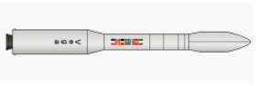
Fig. 1. Launch vehicle Vega (Vettore Europeo di Generazione Avanzata, ASI&ESA) [5]

Within the framework of this study we shall consider a light launch vehicle which has been jointly developed by the European Space Agency (ESA) and the Italian Space Agency (ASI) since 1998 (Fig.1) [5]. It is qualified to launch satellites ranging from 300 kg to 2000 kg into low circular polar orbits. As a rule, these are low cost projects conducted by research organizations and universities monitoring the Earth in scientific missions as well as spy satellites, scientific and amateur satellites. The main characteristics of the launch vehicle are given in Table 1. The launch vehicle Vega [6] is the prototype of the vehicle under development.

The planned payload to be delivered by the launch vehicle to a polar orbit at an altitude of ~700 km shall be 1500 kg. The launch vehicle is tailored for missions to low Earth and Sun-synchronous orbits. During the first mission the light class launch vehicle is to launch the main payload, a satellite weighing 400 kg, to an altitude of 1450 km with an inclination of the orbit 71.50⁰.

From the standpoint of the problem concerned, namely the synthesis of the navigational algorithm of the space launcher in the proposed injection sequence we are interested only in the first factor, i.e. accuracy of lifting of the 3rd stage to the point of separation 4th stage. This accuracy, other conditions being equal, is determined by the precision of solving a navigation task in lifting the 3rd stage in consideration of both components: the center of mass and the velocity of the stage. They predetermine the required impulse for the 4th stage [7].

Thus, we may determine the main criterion of the accuracy of the navigation task in relation to the integrated inertial navigation system of the space launch vehicle: we need to ensure maximum accuracy in determining the position and velocity vectors of the 3rd stage of the launch vehicle in the exo-atmospheric phase of the mission in the selected for navigation coordinate system. Clearly, this accuracy, in its turn, other things being equal, depends upon the accuracy of the initial conditions of travel of the 3rd stage, or in other words, the accuracy of navigation on the previous atmospheric phase of the mission [1].

Consequently, in the case of the proposed injection sequence the simplest and most obvious criterion for evaluation of the accuracy of the synthesized system should be adopted. It is required to ensure maximum accuracy in determining the vectors of position and the center -of- mass velocity of the launcher during the flight of the1st-3rd stages, i.e. in atmospheric and exo-atmospheric phases of the mission. This accuracy can be characterized by the value of the dispersions posteriori of the corresponding components of the mentioned vectors [8].

Matherials and Methods. Now let's consider the possible integration schemes for GINS and GPS receiver with respect to this technical problem [9]. As it has been aforementioned, currently we can think of three possible integration schemes as follows [10-14]:

· uncoupled (separated subsystems);

· loosely coupled;

· tightly coupled (ultra-tightly coupled).

Uncoupled systems are the simplest option for simultaneous use of INS and GPS receiver [15]. Both systems operate independently. But, as INS errors constantly accumulate, it is necessary eventually to make correction of INS according to data provided by the GPS receiver. Creating such architecture requires minimal changes to the hardware and the software [9].

In loosely coupled systems GINS and GPS also generate separate solutions, but there is a binding unit in which GPS-based measurements and GINS readouts make assessment of the status vector and make corrections of data provided by GINS [15].

The advantage of this scheme is in high functional reliability of the navigation system. The drawback is in correlation of errors, arriving from SGS to the input of the second Kalman filter and the need of strict synchronization of measurements provided by INS and SGS [15].

In tightly coupled systems (Fig. 2) the role of the INS is reduced only to the measurement of the primary parameters of translational and rotational motions. For this reason, in such systems INS are only inertial measurement units, and the GPS receiver is without own Kalman filter. In such a structure both INS and SGS provide a series of measurements for a common computing unit [15].

Fig. 2. Tightly coupled system using INS and GPS receiver

Tightly coupled systems are characterized by high accuracy compared with aforementioned systems, and the integrated filter makes it possible to use all available GPS satellites optimal way, but at cost of the functional redundancy of the system. Tightly coupled systems use the only "evaluator" (as a rule, the Kalman filter) that uses differences between pseudoranges and/or pseudovelocities, calculated (predicted) by INS and measured by Self-Guided System. Advantages of such a scheme are the following [6]:

· the problem of measurement correlation is absent;

· there is no need in synchronization of INS and Self-Guided System as just one clock generator is used;

· search and selection of law quality measurements of pseudorenges.

The disadvantages of closely coupled systems are the following [6]:

· the need for special equipment for Self-Guided Systems;

· use of complex equations for measurements;

· low reliability because INS failure may result if failure of the whole system.

The later drawback can be eliminated by introducing a parallel Kalman filter only for Self-Guided System [9].

Results and Discussion. The main factors that determine the structure and composition of the navigation system are required accuracy and reliability of navigation parameters within the given limits on the weight, size, power consumption (in some cases - for the time of the system development and operation security) (Table 1). Besides, consideration should be given to:

· types of objects;

· cost of the complex;

· service conditions;

· possibility of maintenance and repair.

Table 1

The main advantages of integrated systems

Factors	Quality characteristic
Accuracy	substantially
Weight	decreasing by 30-70%
Volume	decreasing by 50-60%
Power consumption	decreasing by 25-50%
Reliability	increasing 2 times
Redundancy level	increasing by 50% and more
Cost	substantially

Proceeding from the above information we may conclude that an integrated navigation system of future launchers should have a structure which, depending on the functionability of SGS receiver, shall allow operating in accordance with the algorithms both as an uncoupled and tightly coupled system. It should be capable of processing coordinates and velocities as well as pseudoranges and pseudovelocities.

The structure of the complex is to be open to information from other on-board navigation tools and external consumers of navigation information. This may be done by introducing the corresponding input/output ports.

With regard to the above considerations, we propose the following structure of the integrated complex:

· GINS – the main system that provides self-sufficiency and reliability;

· GPS receiver – a device correcting GINS in latitude, longitude, altitude and velocity in three velocity projection components;

· onboard computer – carries out a full range of programs providing operation in various modes, in particular, it comprises a Kalman filter algorithm.

Clearly, the first of the above schemes using both GINS and GPS receiver is not acceptable for our task, because here the receiver is not used for calibration (adjustment) of GINS during the mission by evaluating the drift component. As a result, in the absence of GPS-data errors of GINS grow at the same rate as in the absence of the receiver [6].

Next, each of the two following schemes of interconnection (uncoupled and tightly coupled) have their advantages and disadvantages with regard to the technical problem in question. Indeed, by using a loosely coupled scheme we can implement evaluation of GINS drift components and therefore in the absence of GPS-data, "departure" of GINS will be significantly compensated. Which means that the apriori rejection of a tightly coupled scheme as the most challenging to implement is not a sufficient reason. Indeed, if the flight conditions allow us to estimate the actual values of systematic errors in measurement of and pseudorange and pseudovelocity, the tightly coupled scheme allows us obtain the highest possible accuracy of navigation [6].

Thus, we conclude that in the present study it is appropriate to examine both schemes of interconnection: tightly and loosely coupled, and based on the results of simulation, draw conclusions in favor of one of the possible solutions. Let us briefly examine the scientific and technical problems arising when making the corresponding models and algorithms.

MM of spatial motion of center of mass and relative to center of mass of a solid launch vehicle is well known and widely described in sources.

Mathematical models of GINS are currently also well described in sources, e.g. [17-21]. At the same time MM of GINS drift depends essentially on the type of gyro units and accelerometers used in GINS. In other words, a so-called nonmodelable constant is always present in the drift model. It ultimately determines the possibility of GINS alignment during flight. Because of apriori uncertainty of this component it is appropriate to select the parameters of the shaping filter in such a way as to ensure the least impact on the accuracy of estimation. In other words, it is advisable in this case to receive a guaranteed result.

MM of the navigation field created by the GPS and GLONASS systems, including the visibility of individual satellites during the flight well characterized as well and can be implemented as it is described in the source [15, 22].

Now we shall move on to the analysis of the possible algorithms for processing navigation information. Due to the specific nature of the set task that requires processing of navigational measurements as soon as they are received, we will consider only the recursive modification of the following algorithms: Bayesian (and Kalman filter) or recurrent modification of the least square method, which do not require, as we know an additional a priori information about the state vector of the object. Thus, measurements generated in GINS enter with a relatively high frequency (200 Hz) while the code measurements from the receiver generally enter with a frequency of 1 Hz and the fact that GPS delay measurements may require special modifications of the recursive information algorithm. Finally, essential is the choice of a model predicting object's motion in the onboard algorithm. Moreover, generally there can be several different prediction models which will be used for different phases of flight: atmospheric and exoatmospheric.

Next, the different prediction models can be used when using loosely coupled scheme of interconnection with the different rates of data entry from the GINS and GPS receiver.

Finally, the last aspect that we need to consider in setting the technical problem in the present paper is selecting an approach to the shaping of an integrated navigation system for a space launch vehicle with GPS technology. It is important to stress once again, as mentioned earlier, the term "shape" will understand the structure, composition, models and algorithms for integrated navigation system [1].

Obviously that with regard to the variety of different physical nature of uncontrolled factors having an effect within the framework of this problem, the nonlinear nature of MM of subject's motion and nonlinear relationship between the results of measurements and navigation components of the state vector, the only reasonable approach to solving the technical problems stated above is the simulation of the operation of the system to be shaped.

The above stated makes it necessary to create a special "tool" that shall ensure the implementation of the chosen approach to the solution of the technical problem set. This tool is a computer system with a fairly simple interface allowing, nevertheless varying interactively source data and parameters of the models and algorithms for analyzing and modeling results presented in graphic and numeric forms. Generally such a system must include two models: a model of the environment and a model of a launcher board [6].

For its part, a model of the environment should include as much detailed model of the object, disturbances, and natural and artificial navigation fields.

Model of a Control System for the Launch Vehicle. A control system of the launch vehicle is designed to maintain the required (programmed) trajectory parameters of the center of mass and around the center of mass (Fig. 3) [16]. The launch vehicle under consideration has only a control system of angular motion, as its flight is conducted under a fixed program changing the pitch angle in time [24].

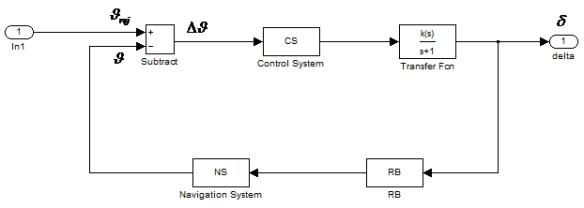
Fig. 3. Control system of the launch vehicle: CS – Control System; RB – Rocket Booster; NS – Navigation System

Thus, control system of the launch vehicle in this case is designed for testing programmed orientation angles of the launch vehicle and attenuation of disturbing environmental influences (wind, disturbing forces and moments in the separation of stages of the launch vehicle, etc.) [1]. Control loop implements program control, i.e. system tends to nullify the difference between the current (variable) and programmed (set in time) orientation angles of the launch vehicle. Thus, the launch vehicle flies in a so-called "fixed" trajectory [24].

Obviously, the initial information for the control loop is based upon measured values of the orientation angles of the launch vehicle and the absolute angular velocity component of the launch vehicle in a body-fixed frame [25, 26].

Physically and logically the control system of the launch vehicle is divided into stages, since, first, different stages use different controls (control thrusters and movable nozzles), and second, weight and inertial characteristics of the launch vehicle vary significantly in different phases of its flight which requires to change the parameters of the control loop integrally.

Besides, the control system is divided by channels (longitudinal and lateral motion) despite the fact that in the first stage control of both channels is performed by the same controls [1].

The parameters of control loop were chosen based on the following conditions: in the boost phase (BPH) generally and in all modes stability of all closed loops in the control system (CS) must be ensured. Accordingly, the author has made programs changing the coefficients which correspond to the controllers of the control system [27].

Accordingly, both loops close with the help of special devices - distributor and limiter of drive signals. Roll control loop of the first stage corresponds to the structure diagram shown in Fig. 4.

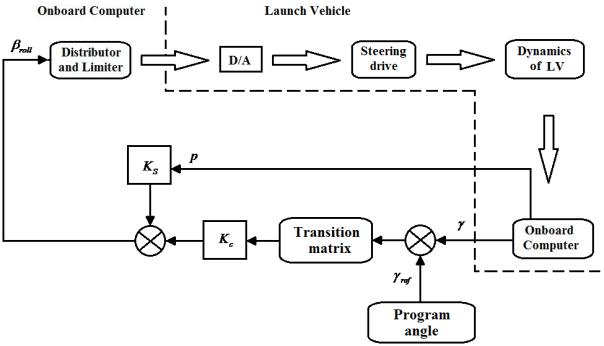
Fig. 4. Structure diagram of the roll control loop for the first stage of the launch vehicle

The master controller equation shall be the following:

Since angular velocities of the launch vehicle are determined in a body-fixed frame and deflections of controls are determined in the same coordinate system, the difference between the angles of orientation of the launch vehicle must be reprojected using the transformation matrix in the following form:

Then, the controller equation may be as follows [24]:

The structural diagram of the limiter is given in Fig. 5.

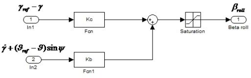
Fig. 5. Structural diagram of the limiter

A simplified mathematical model of the drive is shown in the structural diagram (Fig. 6).

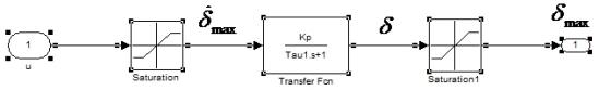
Fig. 6. Simplified mathematical model of the drive

Here: is an input signal; is nozzle deflection;

is a feedback coefficient;

is the time constant of the drive;

are permissible values of the angular velocity and the angle.

Pitch and Yaw control System of the First and Second Stages. The pitch control loop and yaw control loop have the same controllers in the first and second stages. At the beginning the boost phase commands from the controllers are sent to the drives of the first stage only, and then, during the simultaneous operation of the first and second stages for a few seconds commands from controllers are sent to the drives of the first and second stages simultaneously, and after separation of the boosters of the first stage - only to the drives of the second stage.

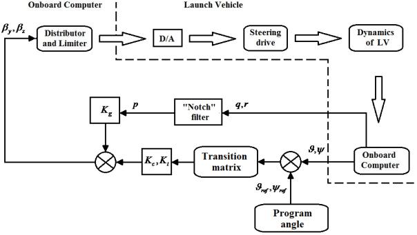
Fig. 7. Structural diagram of pitch and yaw control loop of the first stage of the launch vehicle

The pitch and yaw control loops of the first stage correspond to the structural diagram shown in Fig. 7.

Generation of a control signal for the distributor and the limiter in the first stage is described above.

A distributor is absent in the second stage, and a limiter is used to limit command signals by the maximum specified value of the deflection angle of the nozzle:

pitch signal: if

yaw signal: if

A simplified mathematical model of the drive is presented in the structural diagram (Fig. 8).

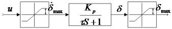
Fig. 8. Simplified mathematical model of the first stage drive

Here: is an input signal; is control deflection;

is a feedback coefficient;

is the time constant of the drive;

are permissible values of the angular velocity and the angle.

Pitch and Yaw Control System of the Third Stage. A limiter is used to limit command signals by the maximum specified value of the deflection angle of the nozzle:

pitch signal: if

yaw signal: if

Roll Control System of the 2nd and 3rd Stages. The main purpose of the roll control loop on the second and third stage is to stabilize the roll movement of the launch vehicle and attenuate any disturbances acting along the trajectory. Unlike in the first two stages, stabilization is achieved by four specialized liquid propellant engines installed diametrically in the third stage and creating control moment pair wise, and not by deflection of nozzle of the solid propellant sustainer engine.

The roll control loop starts with the moment of separation of the first stage and runs until the moment of separation of the third stage.

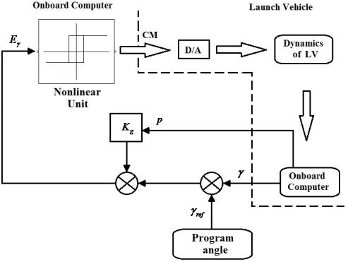
Fig. 9. Structural diagram of roll control loop of the 2nd and 3rd stages of the launch vehicle

Block diagram of the roll control loop for the 2nd and 3rd stages of the launch vehicle is shown in Fig. 9.

Conclusions

1. Based on the above, we have set a technical problem of the conceptual design of an integrated navigation system for the space launch vehicle qualified to inject small artificial Earth satellites into low and medium circular orbits.

2. The conceptual design of the integrated navigation system based on GPS technology involves determination of its structure, models and algorithms, providing the required accuracy and reliability in injecting payloads with due regard to restrictions on weight and dimensions of the system.

3. We have defined the sequence of essential scientific and technical problems that lead to the solution of the major technical problem.

4. It has been demonstrated that it is appropriate to take a posteriori accuracy dispersion of the position and velocity vectors of the launch vehicle in phases of flight of I-III stages as a criterion of accuracy of solving a navigation task.

5. We have made an analysis of possible models of flight and navigation measurements and identified key potential difficulties in the process of their creation.

6. We have shown that the main approach to solving the technical problem is simulation modeling with application of object-oriented soft.

References

1. Zosimovych Nickolay. Integrated Navigation System for Prompting of the Commersial Carrier Rocket. Information technology Conference for Academia and Professionals (ITC-AP 2013), Sharda University, India, 19-21 April, 2013.

2. Flight instruments and navigation systems. Politecnico di Milano - Dipartimento di Ingegneria Aerospaziale, Aircraft systems (lecture notes), version 2004.

3. George M. Siouris. Aerospace Avionics Systems. Academic Press, INC 1993.

4. Kyu Sung Choi. Development of the commercial launcher integrated navigation system the mathematical model, using GPS/GLONASS technique. 52^nd International Astronautical Congress, France, Toulouse, 2001.

5. http://ru.wikipedia.org/wiki/ - Вега (ракета-носитель).

6. Nickolay Zosimovych, Anatoly Voytsytskyy. Disturbed Motion of the Launch Vehicle with Integrated GPS/INS Navigation Systems. "Бъдещите изследвания – 2014" Proc. X International Scientific and Practical Conference, Sofia, 17-25 February, Vol. 49. Technologies. Physics, Sofia: Бял ГРАД-БГ, 2014, PP. 3-9.

7. Лебедев А.А., Аджимамудов Г.Г., Баранов В.Н., Бобронников В.Т. и др. Основы синтеза систем летательных аппаратов. М.: МАИ, 1996, 224 c.

8. Bayley D.J. Design Optimization of Space Launch Vehicles Using a genetic Algorithm, Auburn University, Alabama, 196 pp., 2007.

9. Zosimovych Nickolay. Selecting Design Objectives for an Integrated Guidance System of a Commercial Launch Vehicle with Application of GPS Technologies. The Open Aerospace Engineering Journal, 2013, Vol. 6, PP. 6-19.

10. Scherzinger, B. Precise Robust Positioning with Inertial/GPS RTK Proceedings of ION-GPS-2000, Salt Lake City UH, September 20-23, 2000.

11. Urmson, C., et al, A Robust Approach to High Speed Navigation for Unrehearsed Desert Terrain, Pittsburgh, PA, 2006.

12. Ds. Whittaker, W, Nastro, L., Utilization of Position and Orientation Data for Preplanning and Real Time Autonomous Vehicle Navigation, GPS World, Sept 1, 2006.

13. Daniel J. Biezad Integrated Navigation and Guidance Systems. AIAA Education Series, 1999.

14. John F. Hanaway, Robert W. Moorehead. Space shuttle avionics system, 505 pp., 1989.

15. Управление и наведение беспилотных маневренных летательных аппаратов на основе современных информационных технологий / Под ред. М.Н. Красильщикова и Г.Г. Себрякова. – М.: ФИЗМАТЛИТ, 2003, 280 с.

16. Nickolay Zosimovych, Anatoly Voytsytskyy. Design objectives for a commercial launch vehicle with integrated guidance system. Novus International Journal of Engineering&Technology, Vol. 3, No 4, 2014, PP.7-28.

17. Boulade S., Frapard B., Biard A. GPS/INS Navigation system for launchers and re-entry vehicles-development and adaptation to Ariane 5. ESA GNC, 2003, pp. 57-64.

18. Kelly A.J. A 3D State Space Formulation of a Navigation Kalman Filter for Autonomous Vehicles. CMU Robotics Institute Technical Report CMU-RI-TR-94-19.

19. Alonzo Kelly. Modern Inertial and Satellite Navigation Systems. The Robotics Institute Carnegie Mellon University, CMU-RI-TR-94-15, 1994.

20. Milan Horemuž. Integrated Navigation. Royal Institute of Technology, Stocholm, 2006.

21. Cox, D. B. Jr. Integration of GPS with Inertial Navigation Systems. Institute of Navigation, pp. 144-153.

22. http://satellite-monitoring.at-communication.com/en/secure/seu8800.pdf - Satellite Monitoring and Intercept System SEU 8800.

23. Федосов Е.А., Бобронников в.Т., Красильщиков М.Н., Кухтенко В.И. и др. Динамическое проектирование систем управления автоматических маневренных летательных аппаратов. М.: Машиностроение, 1977, 336 с.

24. Veniamin V. Malyshev, Michail N. Krasilshikov, Vladimir T. Bobronnikov, Victor D. Dishel. Aerospace vehicle control, Moscow, 1996.

25. Zelenkov A.A., Sineglazov V.M., Sochenko P.S. Analysis and synthesis of the discrete-time systems. Kyiv: NAU, 2004, 168 p.

26. Jiann-Woei Jang, Abran Alaniz, Robert Hall, Nazareth Bedrossian, Charles Hall, Mark Jackson. Design of Launch Vehicle Flight Control Systems Using Ascent Vehicle Stability Analysis Tool. AIAA Guidance, Navigation, and Control Conference, 08-11 August 2011, Portland, Oregon, USA. AIAA 2011-6652.

27. Основы проектирования летательных аппаратов (транспортные системы). Учебник для технических вузов / В.П. Мишин, В.К. Безвербый, Б.М. Панкратов и др. Под ред. В.П. Мишина. – М.: Машиностроение, 1985. – 360 с.