ESTIMATION
OF OPTIMAL DEVELOPMENT OF ECONOMY ON THE BASIS OF OPTIMISING MODEL
ImanalievZ.K., BarakovaZ.T.
The problem of
optimal control is investigated for one-grocery model of economy. The new
approach is offered it is based on simple properties of decreasing function on
the closed interval.
Introduction
In many works qualitative researches of
models of economic systems and working out of analytical algorithms of
optimization are based on ideas of sufficient conditions of optimality [1] or
on direct application of a principle of a maximum [2].
Last year’s research of problems of optimal control by a method of the theory
of perturbation [3, 4] is of special interest and thus the great attention is
given to studying of models with smallperturbation which demand high culture theasymptotic analyze . The asymptotic analysis gives the
chance to receive a qualitative picture of the decision and allows to offer
economic computing procedures for the approached decision of initial problems
of the optimal control which decisions are complicated or it is almost
impossible because of nonlinearity, computing
instability, high dimension and etc.
Small perturbationsin problems of optimal control can be entered artificially
and then the theory of perturbationsacts as a method of research of an initial
problem [4]. In this sense it can be applied to studying of the main properties
of trajectories and modes of development of economic system.
In the given article the problem of optimal controlfor
one-grocery model of economyis investigatedwith the method of small parameter
and is carried the comparative analysis with known results which are received
in [1] other ways out.
It is necessary to notice that in the begin of this
problem it is required to form a highway of the given model and to find the
corresponding management realizing this highway. At the decision of the last, there
is the new approach which is based on simple properties of decreasing function
on the closed interval.
1.
The decision of a
problem of management of economy at macro level withlinearfunctional
Let's
consider process of economy which is characterized during each moment of time t
by a set of variablesX,Y,C,K,L,J, where X-intensity
of a national produce, Y - intensity of an end-product, C -
non-productive consumption, J - total capital investments, K -
the size of the capital, L - labor force.
Interdependence of these variables
are defined by following parities:
![]() (1)
(1)
where![]() the amortization factor,
the amortization factor,![]() «small parameter»
«small parameter»![]() characterizes rate of change of the
cash capital. From equation (1) it is received
characterizes rate of change of the
cash capital. From equation (1) it is received
![]() (2)
(2)
where
a ![]() share of non-productive consumption,
share of non-productive consumption,
![]() (3)
(3)
Thesizes of a national produce are defined by the set production function![]() , i.e.
, i.e.
![]() (4)
(4)
It is supposed that production function![]() is continuous and is twice
differentiated and at any positive expenses of factors following parities:
is continuous and is twice
differentiated and at any positive expenses of factors following parities:
![]()
We consider also that return from manufacture scale is constant, i.e.
for any positive number![]() :
:
![]() (5)
(5)
There are considered following
restrictions of the given process at research:
![]() ,
, ![]() ,
,
where![]() - the set level of the capital,
- the set level of the capital,![]() - level of capital during the initial moment of time. Admissible
process is represented set of function
- level of capital during the initial moment of time. Admissible
process is represented set of function![]() which satisfy to conditions (1-5).
which satisfy to conditions (1-5).
Theproblem of management of the given economy consists in that process![]() which would provide the
greatest consumption on an interval of
time [0, T] c with the account of discounting of consumption, i.e.
which would provide the
greatest consumption on an interval of
time [0, T] c with the account of discounting of consumption, i.e.
![]() , (6)
, (6)
Where![]() weighing function,
weighing function,![]() discounting factor.
discounting factor.
Transient time interval we will consider final. Then during the final
moment of time![]() it is necessary to set is minimum
admissible value of the capital to provide possibility of consumption and
outside of the given horizon of time
it is necessary to set is minimum
admissible value of the capital to provide possibility of consumption and
outside of the given horizon of time![]() .
.
We reduce the given problem. For this purpose we will enter relative
variables:![]() - capital size on one worker (capital arms),
- capital size on one worker (capital arms),
![]() - среднедушевое consumption,
- среднедушевое consumption,![]() - labor productivity. We consider that the gain of a manpower occurs to
the constant rate equal
- labor productivity. We consider that the gain of a manpower occurs to
the constant rate equal![]() , then
, then![]() .
.
Let's spend transformation функционала
(6) to relative variables:
![]() (7)
(7)
Or
![]() .(7)
.(7)
Then the reduced problem can be formulated so: to find such process![]() which delivers a minimum (7) at
restrictions
which delivers a minimum (7) at
restrictions
![]() (8)
(8)
![]() ,
, ![]() ,
,
![]()
![]() (9)
(9)
![]() ,
, ![]() ,
,
where![]()
Let's designate through![]() set of values
set of values![]() satisfying conditions (8), (9) and
we name its admissible area of process.
satisfying conditions (8), (9) and
we name its admissible area of process.
Thesimilar problem in a case![]() is considered in [1].
is considered in [1].
Thegreatestaverage per capitalconsumption
which should be provided by this process is estimated by size functional(7) with a
return sign. In this problem a system condition is ![]() - capital size on one worker,
management - labor productivity
- capital size on one worker,
management - labor productivity![]() and a consumption share
and a consumption share![]() . As the process equation the
differential equation of growth capital armsserves.
. As the process equation the
differential equation of growth capital armsserves.
If to enter "fast" time![]() under the formula
under the formula![]() , where
, where ![]() small parameter then in time
small parameter then in time![]() initial
initial![]() is "slow" time. In that
case, variable factors of investigated system in "fast" time
is "slow" time. In that
case, variable factors of investigated system in "fast" time![]() will appear slowly changing.
Introduction in system of small parameter
will appear slowly changing.
Introduction in system of small parameter![]() is a certain idealization which
underlines that rate of course of process above (approximately,
is a certain idealization which
underlines that rate of course of process above (approximately,![]() time increases), than in a usual
mode.
time increases), than in a usual
mode.
Let the sizes of an end-product are defined by production function of
Kobba-Duglas [1, 5]. Then labour productivity![]() is defined by function
is defined by function
![]()
![]() , (10)
, (10)
Where![]() - factor defining rate of increase
of technical process,
- factor defining rate of increase
of technical process,![]() - factor of elasticity of release
on production assets;
- factor of elasticity of release
on production assets;![]() - factor of elasticity of release
on work.
- factor of elasticity of release
on work.
Theequation (8) taking into account (10) registers in a
kind:
![]() . (11)
. (11)
Let's consider a problem (7), (11), (9). We will enter
new function
![]() . (12)
. (12)
Then taking into account (12) from (11) we will have:
![]() .(13)
.(13)
Now from the right part (13) we will exclude![]() . Wewilldemand, thatthesumfacing
. Wewilldemand, thatthesumfacing![]() , i.e. function
, i.e. function
![]()
Did not depend from k. Then
![]() .
.
Let's have from here:
![]() (14)
(14)
Or
 . (15)
Taking into account (12) equation (13) it is possible
to give a kind
![]() .(16)
.(16)
Then taking into account (14) from (16) we will
receive:
![]() .(17)
.(17)
Taking into account (14)functional(7) it is possible to write down in
a kind:
![]() . (18)
. (18)
Considering (15) of (12) we will have:
 (19)
(19)
 .
.
From the formula (19) we will find:
![]() . (20)
. (20)
Comparing the equations (17), (20) we will receive:
![]() . (21)
. (21)
The condition (21) takes place, if
 .(22)
.(22)
Similarly in [1], function![]() (15) we name a highway of the given
dynamic model. The management realizing this highway - a constant which is
defined by a parity (22). Thentakingintoaccount (22) parity (18) registersin a
kind:
(15) we name a highway of the given
dynamic model. The management realizing this highway - a constant which is
defined by a parity (22). Thentakingintoaccount (22) parity (18) registersin a
kind:
 .
.
Here subinterval function![]() - the discounted size of the
capital.
- the discounted size of the
capital.
From (19) it is visible that at![]() function
function![]() - decreasing on a piece
- decreasing on a piece![]() , and
, and![]() is its greatest value, i.e.
is its greatest value, i.e.
 .
.
Thus
 .
.
At![]() function
function![]() increasing on a piece
increasing on a piece![]() Then
Then
 ,
,
 (23)
(23)
At![]() we will have
we will have
![]() (24)
(24)
In "fast" time a![]() highway
highway
 (25)
(25)
It will appear slowly changing functions.
At![]() ,
,![]() have following limiting values:
have following limiting values:
 ,
,
![]()
For short time intervals change of "slow" variables does not
affect the fast equations and therefore limiting values![]() can serve asymptotical
approach at formation of a highway and gives the chance to receive its
qualitative picture.
can serve asymptotical
approach at formation of a highway and gives the chance to receive its
qualitative picture.
That process![]() , was optimum in sense of a task in
view the decision
, was optimum in sense of a task in
view the decision![]() should satisfy the set regional
conditions (9). But it not so, the decision
should satisfy the set regional
conditions (9). But it not so, the decision![]() cannot satisfy to regional
conditions (9) as through these points take place other curves which are
private decisions of the initial equation (11) at the set management
cannot satisfy to regional
conditions (9) as through these points take place other curves which are
private decisions of the initial equation (11) at the set management![]() .
.
Let's define these curves and their points of intersection with a
highway (a switching point)![]() .
.
Having divided both parts of the differential equation (5) on![]() it is had:
it is had:
![]() .
.
Let's enter a new variable
![]() . (26)
. (26)
Then with the account (25) from (24) we will receive:
![]() .(27)
.(27)
At known![]() (
(![]() - a constant) the exact decision
(27) with the entry condition
- a constant) the exact decision
(27) with the entry condition ![]() registers in the form of the formula
of Koshi:
registers in the form of the formula
of Koshi:
Or
 (28)
(28)
Where![]() .
.
Thedecision of the equation (27) with the entry condition is similar![]() is defined by a parity:
is defined by a parity:
 (29)
(29)
Let's notice that if for the given problem to construct function of
Hamilton then it will depend on management![]() linearly and its maximum values are
reached only in boundary values
linearly and its maximum values are
reached only in boundary values![]() . But in real economic problems as
it is noted in [1], the consumption minimum level is strictly positive:
. But in real economic problems as
it is noted in [1], the consumption minimum level is strictly positive:![]() . Therefore Gamiltonian accepts the
maximum values in points
. Therefore Gamiltonian accepts the
maximum values in points![]() and through these values it is
possible to define switching points.
and through these values it is
possible to define switching points.
Fodefinitions of a point of intersection of a highway with borders of admissible
area![]() it is had following parities:
it is had following parities:
 , (30)
 , (31)
Where![]()
![]() .
.
In formulas (30), (31) if![]() that undertakes the bottom limit
that undertakes the bottom limit![]() , if
, if![]()
![]() . Then the left and right points of
switching are calculated by following formulas:
. Then the left and right points of
switching are calculated by following formulas:
 ,
,
 .
.
Borders of admissible area![]() are defined by parities (28), (26)
at values
are defined by parities (28), (26)
at values![]() . We will put
. We will put![]() . Then the highway
. Then the highway![]() (15) passes how is shown in
drawing. Apparently from drawing, the optimum trajectory consists of three
sites with the moments of switching
(15) passes how is shown in
drawing. Apparently from drawing, the optimum trajectory consists of three
sites with the moments of switching![]() and
and![]() . Since the moment
. Since the moment![]() till the moment
till the moment![]() development goes on a highway, and
out of an interval
development goes on a highway, and
out of an interval![]() consumption is at the bottom level
consumption is at the bottom level![]() , i.e. in these time intervals in
economy there is an accumulation process.As we have noticed above that the
small parameter is entered is artificial in system that as a result we have
received the simplified algorithm which will allow us to offer economic
computing procedures. Therefore it is necessary for us to deduce corresponding асимптотические formulas which give possibilities to construct an optimum trajectory
with certain accuracy, keeping thus qualitative features of studied processes.
, i.e. in these time intervals in
economy there is an accumulation process.As we have noticed above that the
small parameter is entered is artificial in system that as a result we have
received the simplified algorithm which will allow us to offer economic
computing procedures. Therefore it is necessary for us to deduce corresponding асимптотические formulas which give possibilities to construct an optimum trajectory
with certain accuracy, keeping thus qualitative features of studied processes.
Passing by "fast" time![]() we will make variable replacement
in (27):
we will make variable replacement
in (27):
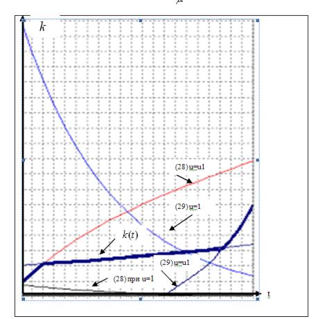
Drawing. An optimum trajectory with the switching moments
![]()
![]() . (32)
. (32)
The
decision of the equation (32) at the known![]() looks like:
looks like:
![]() . (33)
. (33)
For![]()
![]() from (27) we will have:
from (27) we will have:
![]()
![]() . (34)
. (34)
Thedecision (34) registers in a kind:
![]() . (35)
. (35)
Then we have following asymptoticthe
formulas defining points of intersection of a highway with borders of
admissible area![]() :
:
![]()
![]() .
.
Thus the highway is defined from (15), i.e. limiting value undertakes![]() at
at![]() :
:

where![]()
![]() .
.
It is necessary to notice that the first composed in
formulas (33), (35) are accordingly left and right «boundary functions» [4]
which approximate transition from an initial condition on a highway and
transition from a highway in a final condition.
The conclusion
As shows results of the comparative
analysis, conducting small parameter and research of a problem of optimum
control by a method of small parameter allows:
To To receive the simplified algorithm of the decision of
a problem which reduces volume of computing works in 5 … 6 times;
To To define speed of change of the cash capital on one worker and to
receive an estimation of influence of small parameter on changes of the moments
of an exit on a highway.
LIST OF REFERENCES
1. Bases of the
theory of optimum control./ Under the editorship of V.F.Krotova. - М: the Higher school, 1990. - 430 with.
2. Pontrjagin of h.p., Boltjansky
Century Г, Gamkrelidze R. V, MishchenkoE.F.mathematical the theory of optimum
processes. - М: the Science, 1969. - 384 with.
3. Vasileva A.B., Butuzov V. F.
Asimptotichesky decomposition of decisions of the singuljarno-revolted
equations. - М: the Science, 1973. - 272 with.
4. Vasileva A.B.,
DmitrievM.G.Singuljarnye of indignation in optimum control problems//Results of
a science and technics. Sulfurs.Матем. The analysis.-Т. 20.- М: ВИНИТИ, 1982. - with. 3-77.
5. Intriligator of M.
Mathematical methods of optimisation and the economic theory. - М: Progress, 1975. - 606 with.