Экономические науки/4.
Инвестиционная деятельность и фондовые рынки
Doctor of Economics
Sergey N. Yashin
Nizhny Novgorod State
Technical University n.a. R.Y. Alekseev, Russia
Ph.D. in Economic Egor
V. Koshelev
Lobachevsky State
University of Nizhni Novgorod, Russia
Sergey A. Makarov
Nizhniy Novgorod Management Institute of the Academy
of Public Administration under the President of the Russian Federation, Russia
EQUITY RISK MANAGEMENT USING
SYNTHETIC STRADDLES
Equity
risk management primarily implies managing a portfolio of shares and bonds
owned by an investor. In spite of availability of all kinds of financial instruments
reducing such risk, this problem has not yet been fully resolved. One type of
such financial instruments includes derivatives issued for primary (classical)
securities. The reason for which investors continuously develop new financial
instruments reducing equity risk consists in the fact that most derivative
securities require quite an exact prediction of prices for basic assets, i.e.
primary securities. Despite rather a high mathematical exactness of securities
price variance forecasts, their results are to a large extent dependent on
subjective qualities of experts. For that reason, prices for derivative
securities as well as prices for combinations of different securities during
portfolio construction cannot fully reflect actual future changes in their
rates, and these estimates are in many respects of subjective nature.
On the
other hand, investors also make their forecasts which enable them to form their
own opinion on to what extent prices for derivative financial instruments
correspond to their visions of future investment opportunities. That is why,
investors will always go after new options of combining primary securities
using their own methods to reduce their risks. In this regard, it should be
noted that investors have their own visions of the presence and magnitude of
such risks.
One of
the classical derivative financial instruments is an option. Conventional
construction of an option contract implies determination of a striking price. A
striking price means a price to be paid for a basic asset (share) at exercising
the option. Those options that already circulate in the securities market have
their own striking price. It cannot be changed. However, an investor may disagree
that a striking price will really reflect the actual market price per share as
of the time of exercising the option. Certainly, this is the cause of buying or
selling options in the market. But at the same time, an investor faces the
following controversy:
An
option having a certain striking price has a corresponding market price which
is dependent both on the risk related to a specific share and the striking
price. But in view of respective future share price fluctuations, these
fluctuations will in future actually occur not relative to the striking price,
but relative to the actual anticipated share price if the forecast has been
made precisely enough.
This
controversy contributes to investors' going after new combinations of primary
securities which to a greater degree reflect future forecasts according to estimates
of the same investors.
Under
such conditions, we propose a model for constructing a combination of synthetic
options (synthetic straddles) which will enable investors to reduce their equity
risks.
Synthetic
instruments are such instruments that are created by combining other
instruments in such a way as to reproduce the aggregate money flows created by
real instruments.
In case
of a straddle, an option buyer purchases (or sells) both a put option and a
call option for one and the same basic asset (share) with the same striking
price and the same expiration date. In such straddle, an option buyer pays the
seller an amount equivalent to the value of the two options (call and put).
In such
a manner, let us build a synthetic straddle, i.e. a call-put option with the
same striking price using a binomial model [2]. The Black-Scholes model, which
is regarded as a classical model, cannot be used for this purpose for the
reason that a synthetic straddle provides for investor's combining a share
under review and a risk-free bond in its portfolio, whereas the Black-Scholes
model contains a risk-free interest rate only, but no risk-free bond.
For
convenience of further considerations, let us introduce certain designations:
![]() - current market
price per share;
- current market
price per share;
![]() - current anticipated
price per share;
- current anticipated
price per share;
![]() - six-month growth
rate of current anticipated price per share in case of its increase;
- six-month growth
rate of current anticipated price per share in case of its increase;
![]() - six-month growth
rate of current anticipated price per share in case of its decrease;
- six-month growth
rate of current anticipated price per share in case of its decrease;
![]() - anticipated price
per share in six-month period in case of its increase;
- anticipated price
per share in six-month period in case of its increase;
![]() - anticipated price
per share in six-month period in case of its decrease;
- anticipated price
per share in six-month period in case of its decrease;
![]() - anticipated price
per share in twelve-month period in case of its two-fold increase;
- anticipated price
per share in twelve-month period in case of its two-fold increase;
![]() - anticipated price
per share in twelve-month period in case of its increase in six-month period
and decrease in another six-month period;
- anticipated price
per share in twelve-month period in case of its increase in six-month period
and decrease in another six-month period;
![]() - anticipated price
per share in twelve-month period in case of its decrease in six-month period
and increase in another six-month period;
- anticipated price
per share in twelve-month period in case of its decrease in six-month period
and increase in another six-month period;
![]() - anticipated price per share in twelve-month period in case
of its two-fold decrease;
- anticipated price per share in twelve-month period in case
of its two-fold decrease;
![]() - synthetic straddle
striking price in twelve-month period;
- synthetic straddle
striking price in twelve-month period;
![]() - synthetic call
option price;
- synthetic call
option price;
![]() - synthetic put
option price;
- synthetic put
option price;
![]() - synthetic straddle
price;
- synthetic straddle
price;
![]() - synthetic straddle
price in six-month period in case of an increase in anticipated price per share;
- synthetic straddle
price in six-month period in case of an increase in anticipated price per share;
![]() - synthetic straddle
price in six-month period in case of a decrease in anticipated price per share;
- synthetic straddle
price in six-month period in case of a decrease in anticipated price per share;
![]() - synthetic straddle
price in twelve-month period in case of two-fold increase in anticipated price
per share;
- synthetic straddle
price in twelve-month period in case of two-fold increase in anticipated price
per share;
![]() - synthetic straddle
price in twelve-month period in case of an increase in anticipated price per
share in six-month period and a decrease in another six-month period;
- synthetic straddle
price in twelve-month period in case of an increase in anticipated price per
share in six-month period and a decrease in another six-month period;
![]() - synthetic straddle
price in twelve-month period in case of a decrease in anticipated price per
share in six-month period and an increase in another six-month period;
- synthetic straddle
price in twelve-month period in case of a decrease in anticipated price per
share in six-month period and an increase in another six-month period;
![]() - synthetic straddle
price in twelve-month period in case of two-fold decrease in anticipated price
per share;
- synthetic straddle
price in twelve-month period in case of two-fold decrease in anticipated price
per share;
![]() - number of a
six-month period;
- number of a
six-month period;
![]() - current market
value of risk-free bond;
- current market
value of risk-free bond;
![]() - six-month risk-free
interest rate (six-month yield to maturity of risk-free bond);
- six-month risk-free
interest rate (six-month yield to maturity of risk-free bond);
![]() - anticipated price
per risk-free bond in six-month period;
- anticipated price
per risk-free bond in six-month period;
![]() - anticipated price
per risk-free bond in twelve-month period;
- anticipated price
per risk-free bond in twelve-month period;
![]() - number of shares
circulated at present time (
- number of shares
circulated at present time (![]() );
);
![]() - number of bonds
circulated at present time (
- number of bonds
circulated at present time (![]() );
);
![]() - number of shares held
in six-month period (
- number of shares held
in six-month period (![]() ) in situation
) in situation ![]() ;
;
![]() - number of bonds
held in six-month period (
- number of bonds
held in six-month period (![]() ) in situation
) in situation ![]() ;
;
![]() - number of shares
held in six-month period (
- number of shares
held in six-month period (![]() ) in situation
) in situation ![]() ;
;
![]() - number of bonds
held in six-month period (
- number of bonds
held in six-month period (![]() ) in situation
) in situation ![]() .
.
With a
view to illustrating a model construction, let us consider ordinary shares of
Sberbank of Russia. According to information [5], the market value dynamics of
these shares for a twelve-month period is of the nature as shown in Figure 1
and Table 1.
Volume Sberbank of Russia: Set period: Current year 10D Period: May May March March November November September September July 4, 2010 – June 25,
2011 July 4, 2010 – June 25,
2011
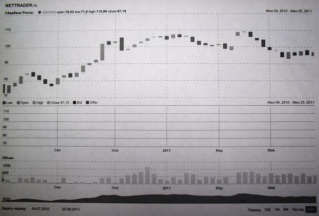
Figure 1. Price Behavior of Sberbank of Russia
Ordinary Shares (RUB)
Table 1. Price Behavior of Sberbank of Russia Ordinary
Shares (RUB)
|
Date |
4.07.10 |
11.07.10 |
18.07.10 |
25.07.10 |
1.08.10 |
8.08.10 |
|
Price |
72.82 |
77.27 |
80.51 |
83.34 |
84.53 |
83.57 |
|
Date |
15.08.10 |
22.08.10 |
29.08.10 |
5.09.10 |
12.09.10 |
19.09.10 |
|
Price |
80.98 |
78.81 |
76.33 |
81.38 |
83.36 |
83.21 |
|
Date |
26.09.10 |
3.10.10 |
10.10.10 |
17.10.10 |
24.10.10 |
31.10.10 |
|
Price |
84.38 |
88.04 |
89.9 |
91.67 |
102.55 |
99.74 |
|
Date |
7.11.10 |
14.11.10 |
21.11.10 |
28.11.10 |
5.12.10 |
12.12.10 |
|
Price |
103.05 |
97.45 |
98.67 |
101.24 |
103.12 |
104.87 |
|
Date |
19.12.10 |
26.12.10 |
2.01.11 |
16.01.11 |
23.01.11 |
30.01.11 |
|
Price |
106.35 |
106.44 |
104.05 |
107.23 |
105.19 |
107.4 |
|
Date |
6.02.11 |
13.02.11 |
20.02.11 |
27.02.11 |
6.03.11 |
13.03.11 |
|
Price |
103.39 |
99.15 |
100.91 |
98.77 |
101.1 |
98.62 |
|
Date |
20.03.11 |
2.04.11 |
9.04.11 |
16.04.11 |
23.04.11 |
30.04.11 |
|
Price |
99.14 |
108.1 |
108.42 |
106.17 |
103.63 |
99.91 |
|
Date |
7.05.11 |
14.05.11 |
21.05.11 |
28.05.11 |
4.06.11 |
11.06.11 |
|
Price |
96.43 |
97.69 |
95.44 |
96.6 |
95.66 |
98.32 |
|
Date |
18.06.11 |
25.06.11 |
|
Price |
96.23 |
96.35 |
The apparent trend in Sberbank of
Russia share price represented by the numerical values in Table 1 and the graph
in Figure 1, despite its general positive dynamics, makes it impossible to obtain
an unambiguous statement as to what extent it will be preserved in future. In
addition, it is not clear whether it will maintain the mean value of share
price fluctuations measured, for instance, by using mean-square deviation
relative to the general trend in share price increase determined, for instance,
by using an equation of linear regression. It is also rather difficult to
determine expressly whether the mean value of share price fluctuations will
remain unchanged in future, or it will be subject to change, i.e. decrease or
increase.
All the specified issues make it
difficult to build classical options reflecting the share price variations to a
greater or lesser extent. Let us resolve such problem by constructing synthetic
straddles.
Using
the figures from Table 1, it is possible to form linear regression of a share
value:
![]() ,
,
where ![]() - price of Sberbank of Russia ordinary share, and
- price of Sberbank of Russia ordinary share, and ![]() - number of a month
starting from 0, i.e. from the date of 4.07.10.
- number of a month
starting from 0, i.e. from the date of 4.07.10.
Let us take a planning time-frame
equal to twelve months. According to the formed regressional relationship, the
striking price as of 25.06.12 will be K,
which corresponds to ![]() RUB.
RUB.
In
doing so, we will adjust our position in the portfolio six months from the
present time, i.e. from the date of 25.06.11 which corresponds to the month of ![]() .
.
In our
binomial model, we assume that the anticipated price per share ![]() RUB determined as of
25.06.11 based on the regression obtained will either grow by 50% (rate
RUB determined as of
25.06.11 based on the regression obtained will either grow by 50% (rate ![]() ) or remain unchanged (rate
) or remain unchanged (rate ![]() ) in the nearest year. Such price variation limits are
selected in accordance with potential yearly inflation rates in Russia.
) in the nearest year. Such price variation limits are
selected in accordance with potential yearly inflation rates in Russia.
Now we
can determine the six-month rate i of
anticipated price growth:
![]() ,
, ![]() ,
,
consequently, ![]() .
.
As a result, the price of the share
under review for the year then ended will change so as shown in Figure 2. It
should be noted that at the moment we use in our calculations the current market
price per share ![]() as of 25.06.11. Moreover,
the situations
as of 25.06.11. Moreover,
the situations ![]() and
and ![]() are identical.
are identical.
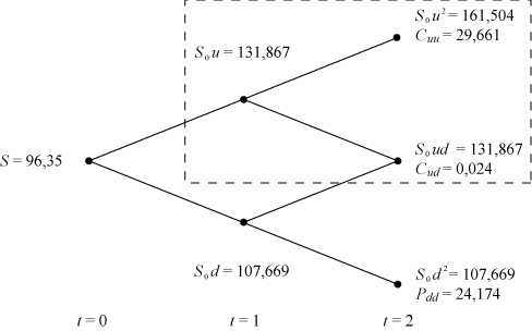
Figure 2. Sberbank Shares Price in Binomial Model
As a risk-free interest rate in
Russia, one may use, for instance, a refinancing rate which accounts for 8.25%
from 3.05.11. However, if we wish to use a risk-free bond in our portfolio,
then it is required to pick up a governmental bond having similar yield to
maturity. This may be, let us say, the OFZ-26205 bond having the yield to
maturity of 8.28% and the real market value of ![]() RUB as of 24.06.11
[4].
RUB as of 24.06.11
[4].
Then we
can find the six-month yield to maturity ![]() :
:
![]() ,
, ![]() ,
,
and ![]() RUB and
RUB and ![]() RUB.
RUB.
In our example, we build a synthetic
option (straddle) which enables its holder either to buy or sell the share
(call-put option) at the end of two six-month periods at the striking price of ![]() RUB. An option that
may be selectively used as a call option or a put option promises at the time
of
RUB. An option that
may be selectively used as a call option or a put option promises at the time
of ![]() contingent money
flows as follows:
contingent money
flows as follows:
![]() ,
,
![]() ,
,
![]() ,
,
![]() .
.
With the figures from our example,
this means that
![]() ,
, ![]() ,
, ![]() .
.
At the moment of ![]() , the call and put option generates neither income nor
expense as it belongs to the European type, which means
, the call and put option generates neither income nor
expense as it belongs to the European type, which means
![]() .
.
To exercise a synthetic option ahead
of time (American option) is irrational since the adjustments in our position ![]() result in
determination of the initial portfolio structure
result in
determination of the initial portfolio structure ![]() , consequently, they are necessary. Otherwise, if we now invest
funds in a portfolio which will not be eventually used, we will sustain damages
in future.
, consequently, they are necessary. Otherwise, if we now invest
funds in a portfolio which will not be eventually used, we will sustain damages
in future.
Then let us set up and solve three
equation systems. In doing so, we sort of move backward in time.
1) Let
us examine Figure 2 and focus our attention to the section highlighted with a
dotted line. Let us suppose that we are at the time point of ![]() , and share prices increased up to
, and share prices increased up to ![]() . In this situation, we may be convinced that the share
prices at the time point of
. In this situation, we may be convinced that the share
prices at the time point of ![]() will either increase
up to
will either increase
up to ![]() or decrease to
or decrease to ![]() . At the same time, this means that the call-put option will
generate money flows either in the amount of
. At the same time, this means that the call-put option will
generate money flows either in the amount of ![]() or in the amount of
or in the amount of ![]() .
.
Then it
is necessary, in view of the current conditions, to construct a portfolio
consisting of a share and a bond, which will at the time point of ![]() generate exactly the
same money flows as the call and put option, namely,
generate exactly the
same money flows as the call and put option, namely, ![]() and
and ![]() . If we further consider that the bond at the time point of
. If we further consider that the bond at the time point of ![]() is quoted at the
price of
is quoted at the
price of ![]() , and one period later, it will provide guaranteed return
flows in the amount of
, and one period later, it will provide guaranteed return
flows in the amount of ![]() , then the equation system for determining structural variables
of an equivalent portfolio will be as follows:
, then the equation system for determining structural variables
of an equivalent portfolio will be as follows:
or with the
specific figures from our example:
wherefrom we obtain
the solutions ![]() and
and ![]() .
.
2) The second equation system implies
that the share price ![]() will drop down to the
value of
will drop down to the
value of ![]() . With this provision, the equivalent portfolio should be formed
so that it could take on the value of
. With this provision, the equivalent portfolio should be formed
so that it could take on the value of ![]() at the time point of
at the time point of ![]() while the share price
remains unchanged, and in case of an increase in the share price – the value of
while the share price
remains unchanged, and in case of an increase in the share price – the value of
![]() . Consequently, we obtain as follows:
. Consequently, we obtain as follows:

or with the
specific figures from our example:
which results in
the following solutions: ![]() и
и ![]() .
.
3) Using the both first equation
systems, we have determined the structure of an equivalent portfolio that we
should select for the convenience of duplicating our option at the time point
of ![]() . Naturally, in order to acquire such portfolio at a certain
time point, it is required to make payments. However, since the call-put option
itself causes neither expense nor income at the end of the first period, these
payments should finance (secure) themselves. Therefore, we should select shares
of the securities in the portfolio at the time point of
. Naturally, in order to acquire such portfolio at a certain
time point, it is required to make payments. However, since the call-put option
itself causes neither expense nor income at the end of the first period, these
payments should finance (secure) themselves. Therefore, we should select shares
of the securities in the portfolio at the time point of ![]() in such a way that
any income related to it at the time point of
in such a way that
any income related to it at the time point of ![]() be actually as high
as any expenses required at this time point. This means as follows:
be actually as high
as any expenses required at this time point. This means as follows:
The left-hand member of the first
(second) formula describes return flows from holding the share and bond at the
time point of ![]() provided that the
share price has increased (decreased). The right-hand member contains income
that is required to finance contingent equivalent portfolios at the time point
of
provided that the
share price has increased (decreased). The right-hand member contains income
that is required to finance contingent equivalent portfolios at the time point
of ![]() . In view of the data from the example and the intermediate
results for the structural variables of the equivalent portfolio, this means as
follows:
. In view of the data from the example and the intermediate
results for the structural variables of the equivalent portfolio, this means as
follows:
which will finally
lead to the solutions: ![]() и
и ![]() .
.
Having these figures, we know for sure
what should be done today (![]() ) and later (
) and later (![]() ) so as, through buying and selling shares and bonds, to pose
ourselves in a position that is by no means different from acquiring the
call-put option as related to anticipated money flows. The price of a portfolio
acquired today is as follows:
) so as, through buying and selling shares and bonds, to pose
ourselves in a position that is by no means different from acquiring the
call-put option as related to anticipated money flows. The price of a portfolio
acquired today is as follows:
![]() ,
,
and this figure, so
long as the capital market is free of any arbitrage, should exactly align with the price of ![]() which an investor
will reasonably agree to pay for the call-put option (synthetic straddle).
which an investor
will reasonably agree to pay for the call-put option (synthetic straddle).
Using Table 2, it is possible to
confirm that our solution actually has the desired property of duplicating the
call and put option. We sell without any coverage at the time point of ![]() shares to the number
of 0.573477, and at the same time we buy 0.80453 bonds. Today, this is
connected with net expenses in the amount of 22.382 RUB. Let us consider for
instance what will happen if the share price goes up at the end of one period.
Selling the share without any coverage will bring us to incur expenses in the
amount of
shares to the number
of 0.573477, and at the same time we buy 0.80453 bonds. Today, this is
connected with net expenses in the amount of 22.382 RUB. Let us consider for
instance what will happen if the share price goes up at the end of one period.
Selling the share without any coverage will bring us to incur expenses in the
amount of ![]() RUB, while due to
holding the bond, we will earn income in the amount of
RUB, while due to
holding the bond, we will earn income in the amount of ![]() RUB. Thus, the
balance on income turns out to be equal to
RUB. Thus, the
balance on income turns out to be equal to ![]() RUB. However, we
should concurrently purchase 1 share and sell 1.261776 bonds. That is why, to
purchase the share, we undertake expenditures in the amount of 131.867 RUB,
while the bonds sold without any coverage bring us income in the amount of
RUB. However, we
should concurrently purchase 1 share and sell 1.261776 bonds. That is why, to
purchase the share, we undertake expenditures in the amount of 131.867 RUB,
while the bonds sold without any coverage bring us income in the amount of ![]() RUB. The balance on
expenses turns out to be equal to
RUB. The balance on
expenses turns out to be equal to ![]() RUB, so income and
expenses become quite equal at the time point of
RUB, so income and
expenses become quite equal at the time point of ![]() . No matter how the share price changes in the second period,
due to the bonds sold without any coverage, we incur expenses in the amount of
. No matter how the share price changes in the second period,
due to the bonds sold without any coverage, we incur expenses in the amount of ![]() RUB. If the share
price increases, we will, through selling the share, obtain 161.504 RUB; if,
conversely, the share price remains unchanged, then our profit will only be
131.867 RUB. In the first case, the balance on income happens to be equal to
29.661 RUB, and in the second case – 0.024 RUB. These values are exactly the
same as the money flows which may be expected by a holder of the call-put
option at exactly the same share price behavior.
RUB. If the share
price increases, we will, through selling the share, obtain 161.504 RUB; if,
conversely, the share price remains unchanged, then our profit will only be
131.867 RUB. In the first case, the balance on income happens to be equal to
29.661 RUB, and in the second case – 0.024 RUB. These values are exactly the
same as the money flows which may be expected by a holder of the call-put
option at exactly the same share price behavior.
Table 2. Duplicating a Call-Put Option
|
Number of Assets |
Payments at a
Time Point |
||||||
|
|
|
|
|||||
|
|
|
|
|
|
|
||
|
|
55.255 |
-75.623 |
-61.746 |
0 |
0 |
0 |
0 |
|
|
-77.637 |
80.788 |
80.788 |
0 |
0 |
0 |
0 |
|
|
0 |
-131.867 |
0 |
161.504 |
131.867 |
0 |
0 |
|
|
0 |
126.702 |
0 |
-131.843 |
-131.843 |
0 |
0 |
|
|
0 |
0 |
107.455 |
0 |
0 |
-131.605 |
-107.455 |
|
|
0 |
0 |
-126.497 |
0 |
0 |
131.629 |
131.629 |
|
|
-22.382 |
0 |
0 |
29.661 |
0.024 |
0.024 |
24.174 |
After the current value of a synthetic
straddle becomes known, it is required to determine whether one should buy or
sell the straddle just now in order to gain profits a year later (at ![]() ).
).
Expected straddle profitability is
dependent on the fluctuation of the basic share price. In our example, these
are shares of Sberbank of Russia. The straddle will bring profits if the shares
are very unstable, but it will yield losses if the price is relatively stable.
The payment schedule (solid line in Figure 3) shows what fluctuation should be
so that the long straddle should bring profits.
Gain on
straddle (RUB) long straddle short straddle Share price (RUB)
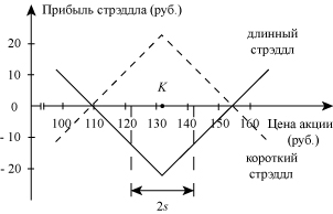
Figure 3. Payment Schedules for a Synthetic Straddle
If at the time of the option
expiration Sberbank's share price is 131.843 RUB, then both call and put
options will end "in the money". Neither option will bring profits,
that is why it will never be exercised, and an investor will incur losses in
the amount of 22.383 RUB.
However, if a favorable situation
occurs, and Sberbank's shares increase in price, for instance, up to 161.504
RUB at the time of the option expiration, an investor will exercise the call option
and earn profits in the amount of ![]() RUB per share. If
taking into account the option value of 22.383 RUB, the investor will earn
RUB per share. If
taking into account the option value of 22.383 RUB, the investor will earn ![]() RUB per share holding
the straddle position. If an unfavorable situation occurs, and the shares sell,
for instance, only at 107.669 RUB at the time of the option expiration, then
the investor will exercise the put option, buy the shares for 107.669 RUB and
resell them to the option seller for 131.843 RUB obtaining income in the amount
of
RUB per share holding
the straddle position. If an unfavorable situation occurs, and the shares sell,
for instance, only at 107.669 RUB at the time of the option expiration, then
the investor will exercise the put option, buy the shares for 107.669 RUB and
resell them to the option seller for 131.843 RUB obtaining income in the amount
of ![]() RUB. In view of
expenses for acquiring the straddle position in the amount of 22.383 RUB, the
investor's profits will be
RUB. In view of
expenses for acquiring the straddle position in the amount of 22.383 RUB, the
investor's profits will be ![]() RUB per share. In
such a manner, a long straddle results in a loss if Sberbank share price is
between
RUB per share. In
such a manner, a long straddle results in a loss if Sberbank share price is
between ![]() RUB and
RUB and ![]() RUB at the time of
the option expiration, but it will yield profits if the share price happens to
be beyond these limits.
RUB at the time of
the option expiration, but it will yield profits if the share price happens to
be beyond these limits.
Consequently, the long straddle
transaction at the time point of ![]() will be only carried
out by those investors who believe that Sberbank's shares will be more unstable
than the fluctuation expectations reflected in the option prices.
will be only carried
out by those investors who believe that Sberbank's shares will be more unstable
than the fluctuation expectations reflected in the option prices.
Investors who believe that Sberbank's
share prices will be less unstable than it was reflected in the option prices
will sell straddles, and this means that they will take on a short straddle position.
The payment schedule for short straddles for Sberbank share options having the
striking price of ![]() RUB and a one-year
maturity period is shown with the small-dotted line in Figure 3. The profit
shaping scheme is exactly opposite to that described above: the straddle seller
earns profits when the share prices are more or less close to the striking
price, but suffers losses when there is a material deviation from it.
RUB and a one-year
maturity period is shown with the small-dotted line in Figure 3. The profit
shaping scheme is exactly opposite to that described above: the straddle seller
earns profits when the share prices are more or less close to the striking
price, but suffers losses when there is a material deviation from it.
Under such circumstances, it is
required to select share price limits at ![]() in respect to which
one should make a decision on what type of synthetic straddles should be built
– a long one or a short one. Such limits at
in respect to which
one should make a decision on what type of synthetic straddles should be built
– a long one or a short one. Such limits at ![]() may be set using a
double standard deviation calculated using the following formulas.
may be set using a
double standard deviation calculated using the following formulas.
1) Average market price per share:
![]() ,
,
where ![]() - market price per
share,
- market price per
share, ![]() - number of epoch of
observation,
- number of epoch of
observation, ![]() - total number of
observations,
- total number of
observations, ![]() - market price per
share at
- market price per
share at ![]() -th epoch of observation.
-th epoch of observation.
2) Unbiased estimator of theoretical
variance:
![]() .
.
As a result, we can find the standard
deviation ![]() .
.
For Sberbank shares, let us calculate
a standard deviation using the figures from Table 1, then let us compare it
with the synthetic straddle price at the time point of ![]() . Finally, we obtain as follows:
. Finally, we obtain as follows:
![]() .
.
Thus, it may be concluded that a
synthetic straddle covers estimated share fluctuation in a twelve-month period
determined by future double standard deviation. Then it is more reasonable for
an investor to build and use in future a short synthetic straddle. This means
that it is required to take actions exactly opposite to the actions described
in Table 2, i.e. to form and adjust the structure of an equivalent portfolio in
such a way that Sberbank of Russia share and OFZ-26205 bond fractions have
signs opposite to the signs obtained in Table 2. This will result in money
flows opposite to those presented in the same table. Using such strategy, an
investor will earn profits on the synthetic straddle a year later.
Consequently, the presented model of
building and using synthetic straddles enables an investor to significantly
reduce its individual equity risk related to its own basic assets, i.e. shares.
This model may be also used to manage other basic assets, such as precious
metals, agricultural commodities (wheat, rice), etc.
References:
1. Brigham E.F., Gapenski
L.C. Intermediate Financial Management. 4th ed. Fory Worth; Philadelphia; San
Diego; New York; Orlando; Austin; San Antonio; Toronto; Montreal; London;
Sydney; Tokyo: The Dryden Press, 1993, vol. 1, pp 245 – 272.
2. Kruschwitz L.
Finanzierung und Investition. R.Oldenbourg; Verlag; Munchen; Wien: R. Oldenbourg
Verlag, 1999. S. 148 – 155.
3. Yashin S.N., Yashina N.I., Koshelev E.V. Innovation and investment companies
financing. Nizhniy Novgorod: VGIPU, 2010, pp 144 – 156.
4. http://quote.rbc.ru/exchanges/demo/micex.1/intraday.
5. http://stocks.nettrader.ru/stocks/securities/list?%5C_init.