Экономические науки/8. Математические методы в экономике
Shevchenko Y.T., doctor of sciences
Bidyuk P.I..
National Technical University of
Ukraine “Kyiv Polytechnic Institute”, Ukraine
Comparative analysis of methods for prediction of
financial processes
Inroduction
Financial processes are difficult to predict and at
the same time it is very important to have a good estimate of the stock prices
forecast.
In last ten years neural networks have received a
great deal of attention in many fields of study [1]. Neural networks are of
particular interest because of its ability to self-train. From a statistical
point of view neural networks are interesting because of their potential use in
prediction problems. They are being used in the areas of prediction where
regression models [2] traditionally being used.
Ward neural net [3], general regression neural net [4]
and polynomial net (GMDH) [5] are of special interest because they show good
results in probabilistic problems.
Statement of
the problem
Let us take the change of quotations of company
Activision Blizzard as an example of financial process and make several
ARIMA-type models and several neural nets to make short-term prediction.
We will make short-term predictions of stock price at
the close of stock exchange using stock price at the opening and indexes NASDAQ
100, S&P 500 (Standard & Poor 500 ) as factors.
The resulting models would be compared by the presence of autocorrelation in the residuals using Durbin–Watson
statistic,
by the proportion of
variability in a data set that is accounted for by the statistical model using coefficient of determination R2, by sum of squared errors. The resulting forecasts
would be compared by mean squared error, mean average percent error and Theil
coefficient.
Theory
3.1 Generalized
Regression Network
A GRN is a
variation of the radial basis neural networks. A GRN does not require an
iterative training procedure as back propagation networks. It approximates any
arbitrary function between input and output vectors, drawing the function
estimate directly from the training data.
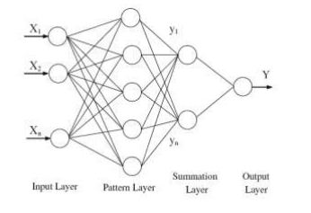
Figure3.1. General Structure of GRN
A GRN consists of
four layers: input layer, pattern layer, summation layer and output layer as
shown in Fig. 3.1. The number of input units in input layer depends on the
total number of the observation parameters. The first layer is connected to the
pattern layer and in this layer each neuron presents a training pattern and its
output. The pattern layer is connected to the summation layer. The summation
layer has two different types of summation, which are a single division unit
and summation units. The summation and output layer together perform a
normalization of output set. In training of network, radial basis and linear
activation functions are used in hidden and output layers. Each pattern layer
unit is connected to the two neurons in the summation layer, S and D summation
neurons. S summation neuron computes the sum of weighted responses of the
pattern layer. On the other hand, D summation neuron is used to calculate
un-weighted outputs of pattern neurons. The output layer merely divides the
output of each S-summation neuron by that of each D-summation neuron, yielding
the predicted value Y0i to an unknown input vector x as ;
![]()
yi is
the weight connection
between the ith
neuron in the
pattern layer and the
S-summation neuron, n
is the number of the
training patterns, D is the Gaussian function, m is the number of
elements of an input vector,
xk and xik are the
jth element of
x and xi, respectively, r is
the spread parameter,
whose optimal value
is determined experimentally.
3.2 Ward network
Ward neural
network - multilayer network, in which the inner layers of neurons are divided
into blocks. These networks are used for solving problems of prediction and
classification.
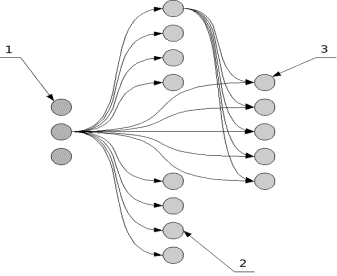
Figure3.1. General Structure of Ward net
Topology of ward
net is
1. The input
layer neurons
2. Neurons of the
hidden layer unit
3. The neurons of
output layer
The partition
into blocks of hidden layers allows to use different transfer functions for the
various units of the hidden layer. Thus, the same signals received from the
input layer, weighed and processed in parallel using multiple methods, and the
result is then processed by neurons in the output layer. The use of different
processing methods for the same data set allows us to say that the neural
network analyzes data from various aspects. Practice shows that the network
shows very good results in solving problems of prediction and pattern
recognition. For the input layer neurons, as a rule, set a linear activation
function. Activation function for neurons of the hidden units and output layer
is determined experimentally.
GMDH
GMDH Network contains in links polynomial expressions. The result of
training is an opportunity to present the output as a polynomial function of
all or part inputs.
The main idea of GMDH is
that the algorithm tries to construct a function (called a polynomial model),
which would behave in such a way that the predicted output value was as close
as possible to its actual value. For many users are very useful to have a model
capable of predicting exercise using familiar and easy to understand polynomial
equations. In the NeuroShell 2 GMDH neural network is formulated in terms of
architecture, called polynomial network. Nevertheless, the obtained model is a
standard polynomial function.
The GMDH algorithm secures an optimal
structure of the model from successive generations of partial polynomials after
filtering out those intermediate variables that are insignificant for
predicting the correct output. Most
improvement of GMDH has focused on the generation of the partial polynomial,
the determination of its structure and the selection of intermediate
variables. However, every modified GMDH
is still a model-driven approximation, which means that the structure of the
model has to be determined with the aid of empirical (regression) approaches. Thus the algorithms could not be said to
truly reflect the self-organizing feature that is able to match the
relationship between variables completely based on the prior knowledge.
The computation experiments.
To construct a prediction for stock prices first of all evaluation
parameters p, q, d for ARIMA-type models were found using auto-correlation and
partical auto-corelation functions. The
time series consisted of 60 observations - daily stock quotes, Blizzard (the
price at the closing).Seven models were built using Eviews 7.0 and Neuroshell 2 software: four
ARIMA-type models and three neural nets. Also indicators of model and
indicators of prediction were calculated to make the comparative analysis of
models: Coefficient
of determination (R2), Sum of squared errors, Durbin –
Watson statistic, mean absolute error(MAE), mean absolute percent error(MAPE),
Theil coefficient.Here is the table with data based on a sample of 60 values:
|
Model Type |
Indicators of model |
Indicators of
prediction |
||||
|
Coefficient of determination R2 |
Sum of squared errors |
Durbin – Watson
statistic |
Mean absolute error |
Mean absolute percent
error |
Theil coefficient |
|
|
Auro-regressive (1,8,9,12) |
0,7074 |
0,9621 |
2,1382 |
0,2108 |
1,7322 |
0,0106 |
|
Auto-regressive with moving average
(1,6,8,9;2,5,7,8,10,11,12) |
0,8402 |
0,3214 |
1,9580 |
0,2734 |
2,24 |
0,0142 |
|
Auto-regressive with trend(1,8,9,12;2) |
0,7252 |
0,9037 |
2,1983 |
0,1891 |
1,5496 |
0,0107 |
|
Auto-regressive with the explanatory
variable(1,6,9,12;2,3,5,8) |
0,8912 |
0,2887 |
2,2383 |
0,1157 |
0,953 |
0,0055 |
|
General regression net |
0,6585 |
1,2 |
1,4474 |
0,115 |
0,9392 |
0,0082 |
|
Ward net |
0,6444 |
1,26 |
1,4451 |
0,118 |
0,964 |
0,0084 |
|
Polynomial net (GMDH) |
0,5064 |
1,722 |
1,1361 |
0,1331 |
1,0814 |
0,0098 |
tab.1
From this table
we can see that neural nets showed worse results than ARIMA-type models.
Results are quite satisfying, but not good enough. So let’s try to build the
same table for sample of 80 values and compare:
|
Model
Type |
Indicators
of model |
Indicators
of prediction |
||||
|
Coefficient of determination R2 |
Sum
of squared errors |
Durbin
– Watson statistic |
Mean
absolute error |
Mean
absolute percent error |
Theil
coefficient |
|
|
Auro-regressive
(AR) |
0,7878 |
1,4157 |
2,1294 |
0,2615 |
2,125 |
0,0129 |
|
Auto-regressive
with moving average (ARMA) |
0,87 |
0,592 |
2,3244 |
0,1474 |
1,197 |
0,0069 |
|
Auto-regressive
with trend |
0,8038 |
1,3085 |
2,1605 |
0,2187 |
1,7814 |
0,0108 |
|
Auto-regressive
with
the explanatory variable (ARMAX) |
0,9367 |
0,2649 |
1,9393 |
0,2471 |
2,0121 |
0,0114 |
|
General
regression net |
0,7998 |
1,36 |
1,519 |
0,107 |
0,8598 |
0,0075 |
|
Ward
net |
0,6517 |
2,4 |
1,106617 |
0,13674 |
1,07298 |
0,00999 |
|
Polynomial
net (GMDH) |
0,8084 |
1,336 |
1,8032 |
0,1065 |
0,863 |
0,0074 |
tab2.
We can see much better results for neural nets on all indicators.
ARIMA-type models showed better results in general, but some indicators of
prediction got slightly worse.
Let’s now take 100 values:
|
Model Type |
Indicators of model |
Indicators of
prediction |
||||
|
Coefficient of determination R2 |
Sum of squared errors |
Durbin – Watson
statistic |
Mean absolute error |
Mean absolute percent
error |
Theil coefficient |
|
|
Auro-regressive (AR)(1,8,9) |
0,769 |
1,9814 |
1,9065 |
0,2554 |
2,0706 |
0,0126 |
|
Auto-regressive with moving average (ARMA) (1,6,8;7,12) |
0,8046 |
1,034 |
1,9803 |
0,2201 |
1,7809 |
0,0105 |
|
Auto-regressive with trend (1,8,9 ;2) |
0,7811 |
1,8782 |
1,912 |
0,2252 |
1,8255 |
0,011 |
|
Auto-regressive with the explanatory
variable (ARMAX) (1,6,8,11;2,4,5) |
0,8712 |
0,7030 |
1,87 |
0,0894 |
0,7236 |
0,0046 |
|
General regression net |
0,7832 |
2 |
1,3285 |
0,115 |
0,9207 |
0,00797 |
|
Ward net |
0,8140 |
1,7 |
1,7053 |
0,105 |
0,8476 |
0,0074 |
|
Polynomial net (GMDH) |
0,8024 |
1,79 |
1,6214 |
0,1127 |
0,9086 |
0,0076 |
tab3.
Comparing with previous sample we see slightly worse indicators of
prediction and better indicators of model, but in general models showed better
results in sample of 80.Let’s take 120 values to find out if results would be
better:
Model Type |
Indicators of model |
Indicators of
prediction |
||||
|
Coefficient of determination R2 |
Sum of squared errors |
Durbin – Watson
statistic |
Mean absolute error |
Mean absolute percent
error |
Theil coefficient |
|
|
Auro-regressive (AR) |
0,7893 |
2,8572 |
2,0608 |
0,1307 |
1,0661 |
0,0066 |
|
Auto-regressive with moving average (ARMA) |
0,836 |
1,5549 |
2,0482 |
0,1969 |
1,6045 |
0,0097 |
|
Auto-regressive with trend |
0,7982 |
2,7362 |
2,0507 |
0,2451 |
2 |
0,0125 |
|
Auto-regressive with the explanatory
variable (ARMAX) |
0,8959 |
1,0453 |
1,9797 |
0,1076 |
0,88 |
0,0055 |
|
General regression net |
0,8018 |
2,76 |
1,6651 |
0,123 |
1,0013 |
0,0087 |
|
Ward net |
0,7946 |
2,88 |
1,6632 |
0,128 |
1,0426 |
0,0089 |
|
Polynomial net (GMDH) |
0,8204 |
2,484 |
1,8795 |
0,1197 |
0,97414 |
0,0083 |
tab.4
The next step is
to determine the best sample: best results during our computations showed
general regression net, worst results showed auto-regressive model. Let’s
compare coefficient of determination and mean absolute percent
error (MAPE) and R- squared for them on different samples:
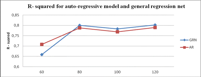
fig.1 R- squared for auto-regressive model and general regression net
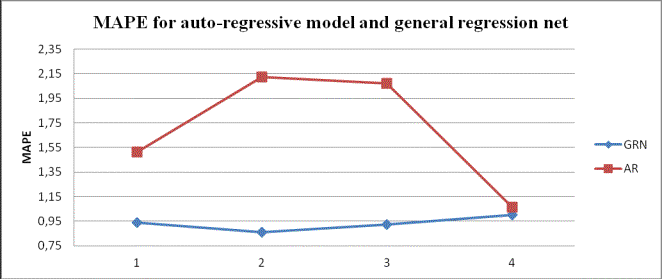
fig.2 MAPE for auto-regressive model and general regression net
According to these two
graphics best results for financial process were obtained with sample of 80
values.
So we found out what sample is best for each process and what models
show best and worse results. Our last step is to make short-term forecast :
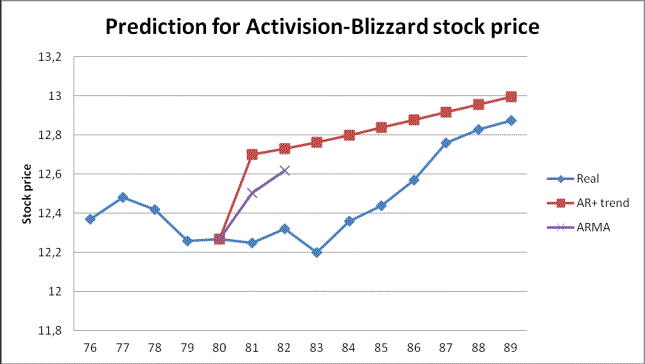
fig.6 short-term prediction for
Blizzard stock price
And the last is one-step prediction
using neural nets and ARMAX:
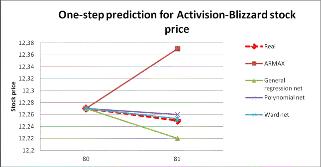
fig.7 One-step prediction for
Blizzard stock price
As we can see neural nets showed very good
results for one – step prediction.
Conclusions
The best results were obtained using general regression net and
polynomial net while the worst results were obtained by auto-regression model.
Analysis of the obtained results of the study shows that in general
forecasted values obtained by neural networks are closer to the
source statistics than results obtained by ARIMA-type models. In our opinion,
this is due to the fact that neural networks designed for application to the
series that have complex and nonlinear structure, while the ARIMA-type models
designed to work with rows that have more noticeable structural patterns.
Literature
1.
Brad Warner, Manavendra Misra Understanding Neural
Networks as Statistical Tools: The American Statistician
Vol.
50, No. 4 (Nov., 1996), pp. 284-293
2.
Бидюк П.И., Романенко В.Д., Тимощук О.Л., Учебное пособие по "Анализу временных рядов" - НТУУ
"КПИ", 2010, 230 с.
3.
Group Method of Data Handling / Web address: http://www.gmdh.net/
4.
GMDH Wiki/ Web address: http://opengmdh.org/wiki/GMDH_Wiki
5.
Donald F. Specht A General Regression Neural
Network: IEEE TRANSACTIONS ON N
E U R A L NETWORKS. VOL. 2 .
NO. 6. NOVEMBER 1991