The technique of tuning the controller parameters on the transient response
of the control object with
automatic compensation
Defining the parameters of the transfer
function, of course, is an important task that requires a serious scientific
approach, which is reflected in the literature [1,2]. This paper describes the
technique of tuning parameters of the controller circuit controls on
experimental transient response.
Initial data: the transition process
and the transition function of the object are given, the transition function of
the object is normalized (Figure 1).
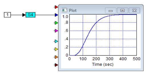
Fig. 1. Initial data of
the transition process
Identification
of the parameters of the transfer function with usage of the transient response
The first
step is to produce identification system to create the model. To do this, find
the point of inflection with the link of differentiation (Figure 2).
From the
graph in Figure 2 the maximum value of the derivative falls on 118.48 s. This
is the point of inflection. Next, you draw a tangent to the transfer function at
the found inflection point (Figure 3). From the figure we can find two time
constants, namely: τ = 65.8 s and T = 146.7 s.
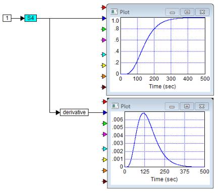
Fig
2. Finding the inflection point with the link of differentiation
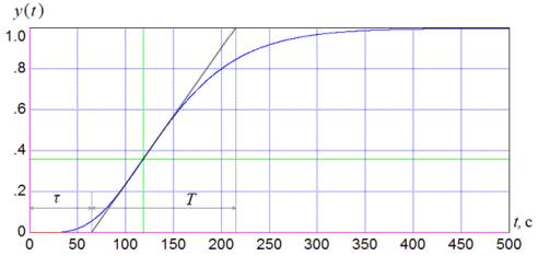
Fig. 3. The tangent to the transfer function at
the inflection point
Find the area S of the figure formed by a given
curve and the transient response of the direct output equal to one (Figure 4).
We can find that S = 150.27.
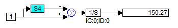
Fig.
4. Finding the area above the curve of the transition function
The
model describing the object with automatic compensation is in the form:
where ![]()
![]()
![]()
Thus, the
scheme of the simulation of the estimated model of the control object will have
the form shown in Figure 5.
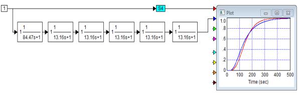
Fig. 5. The scheme
simulation model of the object management
As can be
seen in the Figure 5, the transient response of the original control object and
valuation models are similar with a sufficient degree of accuracy.
Setting up
the PI-controller
Let PI-controller
for the resulting model be set up now. The desired transfer function for open
system is as follows:
Since ![]() , then:
, then:
Suppose
![]() . Then:
. Then:
![]() (4)
(4)
Where ![]() is found from
the formulas (2) and (4).
is found from
the formulas (2) and (4).
The scheme of
simulation of the evaluation model of the system with PI-controller is shown in
Figure 6. The simulation result of the system is shown in Figure 7.
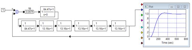
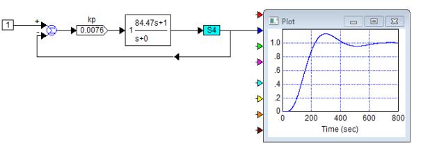
Fig. 6. The scheme of
simulation of the model of the system with PI-controller
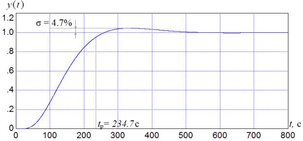
Fig. 7. The result of
simulation of the model of the system with PI-controller
We use the
obtained controller for the original system, but not for its model. The scheme
of the simulation in this case is shown in Figure 8, and the simulation result
is shown in Figure 9.
Fig, 8. The scheme of
the simulation of the original system with PI-controller
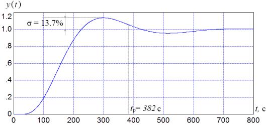
Fig. 9. The result of
simulation of the initial system with PI-controller
Conclusions
In this paper, we have developed the technique of
the setting of the parameters of the controller which was based on the
experimental transient response. It was established the evaluation model of the
control object, and for this model it was designed PI-controller, and then it
was applied to the initial system. According to the simulation results, it is shown
that the transient response became a little worse, because the controller is
not setup to the system itself, but for its evaluation. However, this method
allows you to quickly and with a good quality to design the controller with
automatic compensation for the control object.
References
1. Fradkov, A. L Adaptive management in
complex systems. - Moscow: Nauka. - 1990. - 296 p.
2. Miroschnik, I. V, Nikiforov, V. O., and Fradkov, A. L. Nonlinear and adaptive control
of complex dynamic systems. - St. Petersburg.: Science. - 2000. - 549 p.