Academic of the RANH, corresponding-member of the IAS of HS,

Dr.S. (eng.). Professor,

Pil E.A. Russia, Saint-Petersburg,

THEORY OF THE FINANCIAL CRISES

(PART II)

The author’s earlier articles demonstrated that in order to describe the processes taking place within a country’s economy this economy can be viewed as the volume of the economic shell [1, 2]. This article considers a country’s GDP as the surface area of the economic shell [3, 4, 5, 6].

GDP can be calculated by estimating the surface area S_su, which is affected by external forces P. To perform the calculation, we used four variables, i.e. S_su (GDP_su) = f(Х1, Х2, Х3, Х4). Here we have Х1, Х2, Х3 and Х4, the variables that influence the country’s GDP.

It should immediately be noted that during calculation and plotting of construction drawings, the parameters of X1, X2, X3 and X4 could be constant values, increase or decrease by 10 times. On the basis of the calculations made, 81 graphics were built, which can be divided into the four following groups:

• variable values X1, X2, X3 and X4 increase and are constant;

• variable values X1, X2, X3 and X4 decrease and are constant;

• variable values X1, X2, X3 and X4 decrease and increase;

• variable values X1, X2, X3 and X4 are constant, they decrease and increase.

Figure 1 represents a two-dimensional graph of the dependence S_su (GDP_su), where Х1 = Х2 = Х3 = 1 and Х4 = 0,1…0,99, which shows that the initial values of S_su increase gradually from 14,58 to 23,77 in point 9, and then increase considerably to 102,86, i.e. more than three times 3,22. Figure 2 shows one 3D graph, which allows us to see the changes of S_su more clearly. In this case, it makes sense for us to have the values of the rightmost points, as at these values the value of S_su (GDP_su), i.e. GDP, will be at its maximum. Figure 2 is plotted with the use of variables X3 and X4, i.e. S_su (GDP_su) = f(Х3, Х4).

Figure 1. Dependence S_su (GDP_su) = f(Х1, Х2, Х3, Х4)

when Х1 = Х2 = Х3 = 1, Х4 =0,1…0,99

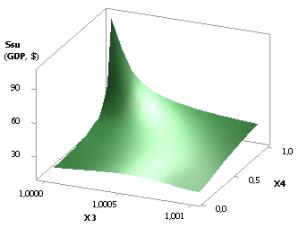
Figure 2. 3D graphic: S_su (GDP_su) = f(Х3, Х4)

when Х1 =Х2 = Х3 = 1, Х4 =0,1…0,99

Figure 3. Dependence S_su (GDP_su) = f(Х1, Х2, Х3, Х4)

when Х1 = Х2 = 1, Х3 = 1…10, Х4 = 0,1…0,99

a	b
c	d

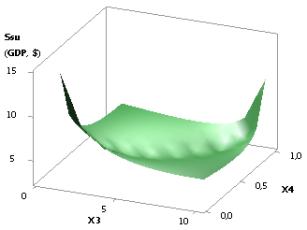
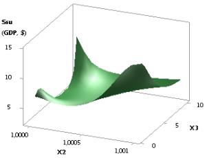
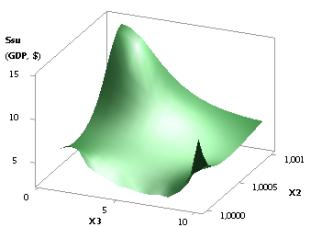
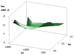
Figure 4. 3D graphics: a - S_su (GDP_su) = f(Х3, Х4); b - S_su (GDP_su) = f(Х2, Х3);

c - S_su (GDP_su) = f(Х3, Х2); b - S_su (GDP_su) = f(Х1, Х4)

when Х1 = Х2 = 1, Х3 = 1…10, Х4 = 0,1

The following Fig. 3 shows that first, at Х1 = Х2 = 1, Х3 = 1…10, Х4 = 0, 1 …0,99, the plotted curve S_su decreases fivefold from 14,58 to the minimum of S_sumin = 2,88 in point 7, and then it drastically increases 3,4 times to 10,29. Figure 4 demonstrates four forms of this dependence as three-dimensional graphs. Here we must note that the form of the 3D graph depends on the choice of the applied axes sequence. For example, in Fig. 4b and 4c we can see 3D graphs with the same variables Х2 and Х3, but with different axes sequences. As we can see, these two graphs’ appearances differ significantly. Based on Fig. 3, it makes sense for us to have the values of the extreme points, as at these values the value of S_su (GDP_su) will be at its maximum.

The plotted curve in Fig. 5 demonstrates that here the values of S_su (GDP_su) at Х1 = Х2 = 1…10, Х3 = 1 and Х4 = 0,99 are rather high, from 102,86 to 102861,38, i.e. they have increased more than 1000 times. Figure 6 shows the plotted 3D graph.

Figure 5. Dependence S_su (GDP_su) = f(Х1, Х2, Х3, Х4)

when Х1 = Х2 = 1…10, Х3 = 1, Х4 = 0,99

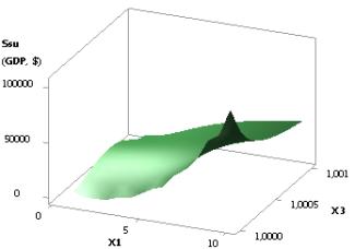
Figure 6. 3D graphic: S_su (GDP_su) = f(Х1, Х3);

when Х1 = Х2 = 1…10, Х3 = 1, Х4 = 0,99

Figure 7 demonstrates the dependence of S_su (GDP_su) at Х1 = 1, Х2 = Х3 = 1…0,1 and Х4 = 0,1…0,99. As we see from the Figure, at first the values of S_su (GDP_su) decrease according to the linear dependence from 14,58 to their minimum of 6,39 at point 9. Then they increase in steps up to 10,29. Figure 8 shows two 3D graphs S_su (GDP_su) = f(Х2, Х1) and S_su (GDP_su) = f(Х1, Х4) respectively. At the given values of the variables, it also makes sense to choose the extreme point values in Fig. 7, which allows us to have the maximum values of S_su (GDP_su).

Figure 7. Dependence S_su (GDP_su) = f(Х1, Х2, Х3, Х4)

when Х1 = 1, Х2 = Х3 = 1…0,1, Х4 = 0,1…0,99

a

b

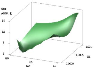
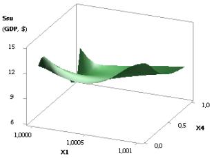
Figure 8. 3D graphics: a - S_su (GDP_su) = f(Х2, Х1); b - S_su (GDP_su) = f(Х1, Х4)

when Х1 = 1, Х2 = Х3 = 1…0,1, Х4 = 0,1…0,99

Figure 9. Dependence S_su (GDP_su) = f(Х1, Х2, Х3, Х4)

when Х1 = 1…10, Х2 = 1…0,1, Х3 = 1, Х4 = 0,99

The following Fig. 9 shows that first the values of S_su here increase from 102,86 to their maximum of 201,64 in point 4, and then they gradually decrease to the value of 10,29, i.e. go down nineteenfold. Figure 10 represents three 3D graphs for S_su (GDP_su) = f(Х2, Х1), S_su (GDP_su) = f(Х3, Х1) and S_su (GDP_su) = f(Х3, Х2) respectively.

a	b
c

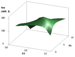
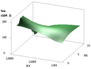
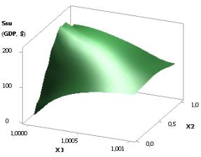
Figure 10. 3D graphics: a - S_su (GDP_su) = f(Х2, Х1); b - S_su (GDP_su) = f(Х3, Х1);

c - S_su (GDP_su) = f(Х3, Х2)

when Х1 = 1…10, Х2 = 1…0,1, Х3 = 1, Х4 = 0,99

In Fig. 11 we can see that the plotted curve S_su (GDP_su) increases gradually from the value of 102,86 to its maximum of S_sumax = 309,72 in point 7, and then it decreases 2,12 times to the value of 145,82. This Figure was plotted at the following values of the variables: Х1 = 1…0,1, Х2 = 1…10, Х3 = 1, Х4 = 0,99…0,1.

For Fig. 9 and 11, it makes sense to choose the values of the variables that are close to their maximum points.

The last Fig. 12 represents four 3D graphs of S_su (GDP_su), and here Figures 12a and 12b, as well as 12c and 12d are plotted with the axes modified.

Figure 11. Dependence S_su (GDP_su) = f(Х1, Х2, Х3, Х4)

when Х1 = 1…0,1, Х2 = 1…10, Х3 = 1, Х4 = 0,99…0,1

After the calculations were made, their results were gathered into a summary Table, which contains 95 lines despite the fact that 81 two-dimensional graphs were plotted. The reason for this is a number of plotted graphs having maximums and minimums.

This summary Table includes such ratios as:

· S_sub…S_suf, where S_sub is the initial value of the economic shell surface area, units²; S_suf is the final value of the economic shell surface area, units²;

· S_suf/S_sub is the ratio of the final value of the economic shell surface area to the initial one.

The ratio of the final value of the economic shell surface area S_suf to the initial one S_sub shows what fold their values increased (decreased) as affected by various external forces. Thus, having these data we can choose the values of the variables Х1, Х2, Х3 and Х4 at which the economic shell surface area will stay unchanged or even increase under the influence of external forces. Thus, during the financial crisis, the selected variable values will allow preserving the country's GDP_su at the same level, or even increasing it.

a	b
c	d

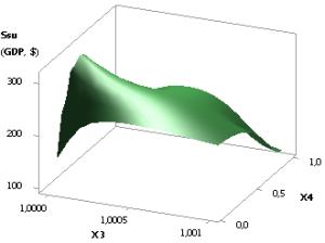
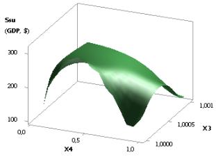
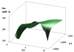
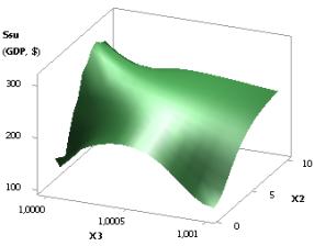
Figure 12. 3D graphics: a - S_su (GDP_su) = f(Х3, Х4); b - S_su (GDP_su) = f(Х4, Х3);

c - S_su (GDP_su) = f(Х2, Х3); b - S_su (GDP_su) = f(Х3, Х2)

when Х1 = 1…0,1, Х2 = 1…10, Х3 = 1, Х4 = 0,99…0,1

After the summary Table with 95 lines was plotted, it was transformed the following way, and only the values where S_suf/S_sub ≥ 1 were left. On the basis of this transformation, we obtained the final summary Table, which included 48 lines. Thus, we obtained 48 variants that allow countries to come out of yet another economic crisis. Below, you can see Table 1, which includes only a part of the summary Table with 22 lines. Here the ratios S_suf/S_sub in the last column are given in descending order.

Table 1 shows that there are two variants at which GDP of a country will not change in the time of an economic crisis, even if we change the variables. These lines are 21 and 22, where the ratios S_suf/S_sub = 1.

Table 1. Statistics of theoretical relation Ssuf /Ssub where Ssuf /Ssub ≥ 1
No. in sequence	Х1, unit	Х2, unit	Х3, unit	Х4, unit	Ssub … Ssuf, unit^2 (GDРsub…GDРsuf), $	Ssuf / Ssub (GDРsuf / GDРsub)
1.	1…10	1…10	1…0,1	0,1…0,99	14,58…1,029E+06	70539,88
2.	1…10	1…10	1…0,1	0,99	102,86…1,03E+06	10000,0
3.	1…10	1…10	1	0,1…0,99	14,58…1,03E+05	7053,99
4.	1	1…10	1…0,1	0,1 …0,99	14,58…1,03E+05	7053,99
5.	1…10	1…10	1	0,99	102,86…1,03E+05	1000,0
6.	1	1…10	1…0,1	0,99	102,86…1,03E+05	1000,0
7.	1	1…10	1	0,1…0,99	14,58…10286,14	705,4
8.	1…10	1	1…0,1	0,99	102,86…10286,14	100,0
9.	1	1…10	1	0,99	102,86…10286,14	100,0
10.	1…10	1	1	0,1…0,99	14,58…1028,61	70,54
11.	1…0,1	1…10	1	0,1…0,99	14,58…1028,61	70,54
12.	1…10	1	1…0,1	0,99…0,1	71,02…1458,20	20,53
13.	1…0,1	1…10	1	0,99	102,86…2016,08	19,60
14.	1	1…10	1	0,99…0,1	102,86…1458,20	14,18
15.	1…10	1	1	0,99	102,86…1028,61	10,0
16.	1	1	1…0,1	0,99	102,86…1028,61	10,0
17.	1	1	1	0,1…0,99	14,58…102,82	7,05
18.	1	1	1…0,1	0,99…0,1	28,75…145,82	5,07
19.	1…10	1	1	0,99…0,1	63,92…145,82	2,28
20.	1…10	1…0,1	1	0,99	102,86…201,61	1,96
21.	1…10	1	1…10	0,99	102,86…102,86	1,0
22.	1…0,1	1	1…0,1	0,99	102,86…102,86	1,0

Now let us transform Table 1 into Table 2, and for this we will group the lines according to the number of variables they include. Thus, Table 2 includes the following four groups: with 1 variable; with 2 variables; with 3 variables and all the variables.

Table 2. The statistics of constant parameters for Ssuf/Ssub in descending order
No. in sequence	Х1, unit	Х2, unit	Х3, unit	Х4, unit	Ssub … Ssuf, unit^2 (GDРsub…GDРsuf), $	Ssuf / Ssub (GDРsuf / GDРsub)
1 variable
1.	1…10	1…10	1…0,1	0,99	102,86…1,03E+06	10000,0
2.	1…10	1…10	1	0,1…0,99	14,58…1,03E+05	7053,99
3.	1	1…10	1…0,1	0,1 …0,99	14,58…1,03E+05	7053,99
2 variables
4.	1…10	1…10	1	0,99	102,86…1,03E+05	1000,0
5.	1	1…10	1…0,1	0,99	102,86…1,03E+05	1000,0
6.	1…0,1	1…10	1	0,1…0,99	14,58…1028,61	70,54
7.	1…10	1	1…0,1	0,99…0,1	71,02…1458,20	20,53
8.	1	1…10	1	0,1…0,99	14,58…10286,14	705,4
9.	1…10	1	1…0,1	0,99	102,86…10286,14	100,0
10.	1…10	1	1	0,1…0,99	14,58…1028,61	70,54
11.	1…0,1	1…10	1	0,99	102,86…2016,08	19,60
12.	1	1…10	1	0,99…0,1	102,86…1458,20	14,18
13.	1	1	1…0,1	0,99…0,1	28,75…145,82	5,07
14.	1…10	1	1	0,99…0,1	63,92…145,82	2,28
15.	1…10	1…0,1	1	0,99	102,86…201,61	1,96
16.	1…10	1	1…10	0,99	102,86…102,86	1,0
17.	1…0,1	1	1…0,1	0,99	102,86…102,86	1,0
3 variables
18.	1	1…10	1	0,99	102,86…10286,14	100,0
19.	1…10	1	1	0,99	102,86…1028,61	10,0
20.	1	1	1…0,1	0,99	102,86…1028,61	10,0
21.	1	1	1	0,1…0,99	14,58…102,82	7,05
all the variables
22.	1…10	1…10	1…0,1	0,1…0,99	14,58…1,029E+06	70539,88

The obtained Table 2 gives us a clear idea that it suffices to change even one variable out of four for the country to successfully come out of an economic crisis.

Thus, depending on the number of variables applied, Table 2 allows us to use a different number of variants:

· with 1 variable (3 variants);

· with 2 variables (14 variants);

· with 3 variables (4 variants);

· all the variables (1 variant).

As we can see, the largest number of variants is available for two variables. However, if we apply all the variables to come out of an economic crisis, in this case we will have the strongest economic effect.

Below you can see Table 3, which shows how much the values of Ssu (GDPsu) change as affected by increase in the number of decimal places for the variable Х4. In other words, this is another variant for a country’s economy to come out of a crisis.

Tables 3. The change of the values of Ssu at the increase in the number of decimal points for the variable X4
No. in sequence	Х1, unit	Х2, unit	Х3, unit	Х4, unit	Ssu, unit.^2 (GDPsu, $)
1	1	1	1	0,9	33,29
2	1	1	1	0,99	102,86
3	1	1	1	0,999	324,54
4	1	1	1	0,9999	1026,06
5	1	1	1	0,99999	3244,63
6	1	1	1	0,999999	10260,39
7	1	1	1	0,9999999	32446,20
8	1	1	1	0,99999999	102603,90
9	1	1	1	0,999999999	324462,02
10	1	1	1	0,9999999999	1026038,96

REFERENCE

1. Pil E.A. Application of the Shell Theory to Describe Processes Taking Place in the Economy. The Almanac of Contemporary Science and Education. 2009. No. 3. P. 137-139.

2. Pil E.A. Theory of the financial crises. International Scientific and Practical Conference. Topical researches of the world science (June 20-21, 2015) Vol. IV Dubai, UAE. – 2015 – Р. 44-56

3. Pil E.A. Calculation of GDP at Constant, Decreasing and Increasing Variables. Materialy XII mezinarodni vedecko-practiсka konference «Veda a technologie: krok do budoucnosti – 2016». 22–28 unora. 2016 roku. Dil 4. Economicke vedy. Administrativa.: Praha. Publishing House «Education and Science» s.r.o. – 88 stran. – P. 10-12

4. Pil E.A. The Influence of Decreasing and Increasing Variables on GDP. Materialy XII mezinarodni vedecko-practiсka konference «Veda a technologie: krok do budoucnosti – 2016» 22–28 unora. 2016 roku. Dil 4. Economicke vedy. Administrativa.: Praha. Publishing House «Education and Science» s.r.o. – 88 stran. – P. 12-14

5. Pil E.A. The Influence of Four Variables on GDP. Materials of the XII International scientific and practical conference, «Modern scientific potential - 2016», February 28 - March 7, 2016 Volume 5. Economic science. Governance. Sheffield. Science and education. LTD. UK – 104 р. – P. 32-35

6. Pil E.A. The Influence of Decreasing and Constant Variables on GDP. Materials of the XII International scientific and practical conference, «Modern scientific potential - 2016», February 28 - March 7, 2016 Volume 5. Economic science. Governance. Sheffield. Science and education. LTD. UK – 104 р. – P. 30-32