About the similarity of particle and photon tunneling and multiple internal reflections in 1-dimensional, 2-dimensional and 3-dimensional photon tunneling.

V.S.Olkhovsky

Institute for Nuclear Research of NASU, Kiev-028, prospect Nauki, 47,Ukraine; olkhovsky@mail.ru

Abstract: The formal mathematical analogy between time-dependent quantum equation for the non-relativistic particles and time-dependent equation for propagation of electromagnetic waves had been studied in [1,2]. Here we deal with the time-dependent Schrödinger equation for non-relativistic particles and with time-dependent Helmholtz equation for electromagnetic waves. Then, using this similarity, the tunneling and multiple internal reflections in 1D (1-dimensional), 2-D and 3-D particle and photon tunneling will be studied. Finally some conclusions and future perspectives for further investigations are presented.

PACS 03.65.Xp; 42.50.Xa

Key words photon tunneling, similarity of photon and particle tunneling, Hartmann phenomemnon, superluminality

I. Introduction. Here we consider the formal mathematical analogy between time-dependent Schroedinger equation for non-relativistic particles and with time-dependent Helmholtz equation for electromagnetic waves and also such similarity of probabilistic interpretation between particle wave function and classic electromagnetic wave packet (being the “wave function of a single photon”, as follows from [1,2]), which is sufficient for the same definition of mean times and durations for processes of propagation, collisions and tunneling of both particles and photons. The only difference in such analogy is caused by linear dependence of energy and impulse for photons and the quadratic dependence of energy from impulse for non-relativistic particles having rest mass. And it induces the physical difference in the spreading of particle wave packets in comparison with photons.

II. Photon tunneling. Concretely let consider hollow narrowed rectangular wave-guide, depicted in Fig.1 (with cross section a ´ b in narrowed part, a < b), which was used for experiments with microwaves [3].

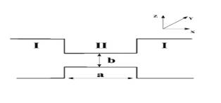
Fig.1. When radio-waves in the microwave range are propagating along the wave-guide, narrowed segment (with cross width which is less than wavelength cutoff) appears as photonic barrier.

Inside it, time-dependent wave equation for any vector , , ( is a vector potential with the additional calibration condition div = 0, = –(1/c) /t is an electric field strength, = rot is a magnetic field strength) has the form

– (1/c² ) ²/t ² = 0. (1)

It is known (see, for instance, [4-6]), that for the boundary conditions

E_y = 0 for z = 0 and z = a , (2)

E_z = 0 for y = 0 and y = b ,

The monochromatic solution (1) can be represented as a superposition of following waves:

E_x = 0 ,

E_y^± = E_o sin(k_z z) cos(k_y y) exp[i(t ± x)] , (3)

E_z^± = –E_o (k_y /k_z ) cos (k_z z) sin(k_y y) exp[i(t ± x)]

(here we have chosen TE-waves) with k_z²+k_y²+²=² /c²=(2/)², k_z = mp /a , k_y =n/b , m and n are integer numbers. Тhus,

g= 2 [(1/)² - (1/_c)²]^1/2, (1/_c)² = (m/2a)² + (n/2b)² , (4)

where is real (= Re), if < _c and is imaginary (= i_em ), if > _c. Similar expressions can be obtained for TH-waves [1,5].

Generally speaking, the solution of equation (1) can be written in the form of wave packet, constructed from monochromatic solutions (3), like the solution of time-dependent Schroedinger equation for non-relativistic particles in the form of wave packet, constructed from the monochromatic waves. Moreover, in representation of the primary quantization, the probabilistic one-photon wave function usually is described by a wave packet for [1,2], for instance,

(,t) = () exp (i- ik_o t) (5)

in the case of plane waves, where ={x, y, z}, ()=k_i ()_i (), _ij =_{i j} , _i ()=0, i,j=1,2 (or y,z, if =k_xx), k_o=/c=e/c, k=||=k_o , k_i () is an amplitude of the probability of possessing by photon the impulse and polarization i and then the quantity |k_i()|²d is proportional to the probability that photon has the impulse in the interval and +d in the polarization state _i. Although it is impossible to localize the photon in the direction of its polarization, nevertheless in a certain sense for one-dimensional motion it is possible to use the space-time probabilistic interpretation (5) along axis x (the direction of motion) [2]. Usually one uses not the probability density and probability flux density on the base of the correspondent continuity equation directly, but the energy density s_o and the flux of energy density s_x (although they represent the components of non 4-vector, but of tensor of energy-impulse) on the base of the correspondent continuity equation [7], which we write in two-dimensional (spatially one-dimensional) lorentz-invariant form:

¶ s_o /t +s_x /x = 0 , (6)

where

s_o =(* + *)/ 8, s_x = c Re [*]_x /2 (7)

and axis x is directed along the motion axis (mean impulse) of wave packet (5).Then, as the normalization condition we choose the equality of spatial integrals s_o and s_x for mean photon energy and mean photon impulse respectively or simply unit flux density for energy s_x. Bypassing the problem of impossibility for the direct spatial probabilistic interpretation (5), we can define conditionally probability density

dx = S_o dx / S_o dx , S_o = s_o dydz (8)

to find (localize) photon in the spatial interval (x,x+dx) along axis x at time t, and probability flux density of

J_em,x dt=S_x dt /S_x dt, S_x =s_x dydz (9)

photon passage through point (plane) x in the time interval (t,t+dt), quite similarly to the probabilistic proprieties for non-relativistic particles. Justification and conditionality of such definitions is supported also by coincidence of the group velocity for wave packet and the velocity of the energy transport which is accepted for electromagnetic waves (at least for plane waves) in [9]. Hence, in a certain sense, in time analysis along the motion direction (1) the wave packet (5) is totally similar to the wave packet for non-relativistic particles and (2) similarly to standard quantum mechanics one can define the mean time of photon (electromagnetic wave packet) passage through point x [8]:

<t(x)> = t J_em,x dt = t S_x(x,t)dt/S_x (x,t)dt , (10)

where for natural boundary conditions k_i (0)=k_i (¥)=0 in energy representation (e=ck_o) one can use the same form of time operator, as for particles in non-relativistic quantum mechanics – and therefore to show the equivalence of calculations for <t(x)>, variance Dt(x) etc in both time and energy representations. Тhen for wave packets like in Fig.1 for the boundary conditions (2) during tunneling the evanescent and anti-evanescent waves with k_x== ± i_em appear. Results (6)-(10) expand the results of [8] for particle tunneling which were recognized to be the best in Copenhagen quantum theory in [10].

In the cases of fluxes which signs are changing we, following [8,11], can introduce quantities J_{em,x, ±} = =J_em,x×( ± J_em,x ) with the same physical sense, as for particles. And then the expressions for mean values and variances of time distributions for moving, tunneling and reflection were obtained in the same way, as for non-relativistic particles in quantum mechanics.

In particular case of quasi-monochromatic wave packets one, using the stationary phase method for particles [12] (when |k_i ()|²d() ) can obtain the similar expression for the phase tunneling time (that is defined in the approximation of the stationary phase)

^Ph _tun,em = 2/c_em for _em L >>1. (11)

From (11) one can see that if _em L > 2, the effective tunneling velocity

v^eff_tun = L /^Ph_tun,em (12)

exceeds c, i.е. is superluminal. It is a particular case of the Hartmann phenomenon which was firstly revealed and studied in [8,13] for 1-D motion of quasi-monochromatic particles, tunneling through potential barriers. Concretely it соnsists in the independency of phase tunneling time on the width of sufficiently wide barrier. This result is consistent with the experimental data [3] for photons.

One can see that for “photonic barriers” electromagnetic waves and photons are tunneling through them similarly to particle tunneling through potential barriers. Tunneling of the classic evanescent electromagnetic waves firstly was studied experimentally in [14] with the utilization of the two-prism scheme (like depicted in Fig.3b). Such barriers were constructed for the study of the electromagnetic-waves propagation in the microwave range through the wave-guides (see Fig.2), in the optical range through devices with the frustrated total reflection (see Fig.3) etc. Further, from [15-19] there are known the results of the optical experiments with tunneling of photons (see the schema from [17], represented in Fig.3а). In Fig.3b there is represented the device with two prisms exhibits the space shift of reflected and transmitted beams with regard of that is expected from the geometric optics [19].

Finally, there are appeared also the experimental works on the study of the generalized Hartmann phenomenon for two barriers ([20,21]). They were performed for the motion (out of the resonances) of the electromagnetic waves in the microwave range through the wave-guards [22] (see Fig.4), as well as for the optical photons in the fibrous optics [23]. Since the tunneling in the both cases was in the region of frequences, far from resonances, the general phase tunneling time was appeared to be independent not only from the barrier widths but also from the distances between the barriers.

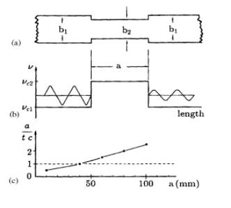
Fig.2. On this scheme there is represented one of the experimental results of Nimtz from [3], accordingly to which the mean velocity of the transmission by the beam of narrow segment exceeds the light velocity с for the sufficiently long “photon barriers”.

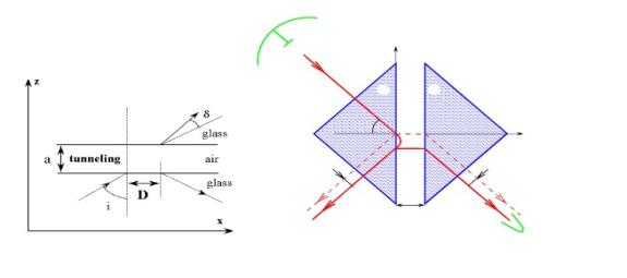
(а) (b)

Fig.3. (а) The violated total internal reflection and tunneling of evanescent waves. (b) Later scheme from [18], considering effect of Goose-Hanchen.

Fig.4. Tunneling of the electromagnecic waves of the microwave range through two narrow segments.

III. The problem of the physical interpretation for the superluminal tunneling velocities of photons. The phenomena of superluminal velocities, observed in the experiments with photon tunneling and evanescent electromagnetic waves [3,15-19] and in number of further works, generated the series of discussions on the relativistic causality, as well as in [3,8,15-19,22-27]etc. Up to now the consensus of the discussion results is not achieved. They are continuing, as well as also the experiments are continuing (see, for instance, [28-30]). Usually now such interpretations of the superluminal tunneling photons are discussed:

1) The interpretation o the superluminal group velocities of tunneling photons without violations of causality or special relativity theory was proposed in [15], started from the reformation (or reconstruction) in the impulse attenuation: later parts of the incoming impulse are attenuated stronger, so in the result the out-coming impulse is shifted to the front parts, effectively intensifying them (and so effectively increasing the group velocity) strictly by causal way. Such scheme is quite compatible with the usual idea of causality (see, for instance, [8]: If the total impulse attenuation is very great and during tunneling the leading part of the pulse is attenuated more less than the cord part, then the time envelope of exit small flux can be completely placed under the initial time envelope of the incoming pulse.

2) It deserves the separate payment the curious idea of “super-oscillations”, proposed in [31].

3) In principle the presence of the superluminal phenomena it is possible, at least partially, to explain also by the non-locality of the barriers, connected with the simultaneous change of the space-time metrics in total inside all the barrier range where energies of incoming wave packets do not succeed the barrier height (more details see in [25,32]).

IV. 1-D tunneling. Аnalysis of multiple internal reflections for the 1-D potentials with the barriers is carrying out during the sufficiently long time (see, for instance, [33-37]). This problem is trivial for the attractive potentials and over-barrier energies inside barriers. And the situation is sharply changing for the under-barrier energies, that is when there is tunneling. In this case evanescent and anti-evanescent waves appear and separately have zero fluxes. To non-zero fluxes there are correspondent only linear combinations of evanescent and anti-evanescent waves together.

For correct analysis of multiple successive reflections from the internal barrier walls during tunneling through it, we shall use the formalism with time analysis of tunneling processes, elaborated in [8], considering also the results of [33-37]. We limit ourselves by the simplest case of the rectangular barrier of the height V₀ in the interval (0, а) along axis x, and the tunneling evolution we shall describe by the non-stationary picture of the actually moving wave packets, соnstructed from the stationary plane waves and being rid of the over-barrier energies by the additional transformation ®Q(E–V₀) (where Q(E–V₀) is the step Heavyside function). Instead of the usual sewing of the stationary wave functions in points x = 0 and x = a for findings of the analytic expressions for A_R , A_{T ,} a and b , we pass to the analysis of the transmission of the initial wave packet through the first wall of the potential barrier, (1) without considering the influence of the second (final) wall of the potential barrier, since the wave packet is not still reached it due to the finite motion velocity, (2) without the violation of the demand of the finiteness for the wave packets in the case of the infinitely wide barriers (since the growing anti-evanescent waves are no introducing still at all), (3) constructing the wave packets by the following steps of the multiple internal reflections in such a way that they were analytic continuation of the appropriate expressions, corresponding to the current waves for the over-barrier energies.

Thus we consider three successive steps in the tunneling evolution:

The first step: A particle initiates the tunneling process through the barrier with the intersection of the first barrier wall at x=0. In this initial step we have the incoming wave packet in the region before the barrier

Y_in (x, t) = dEg(E)y_in(x, k)exp(–iEt/), x< 0 , (13)

plus the wave packet, reflected from the first barrier wall,

(x, t) = dEg(E)(x, k)exp(–iEt/), x< 0 . (14)

The sum of wave packets (13) and (14) does continuously pass after transmission through the initial barrier wall into the wave packet inside the barrier. Supposing the rectangular form and conserving the hypothesis that the tunneling packet does not still feel the second barrier wall, the penetrated under barrier wave packet firstly contains only evanescent waves:

(x, t) = dEg(E)a ₀ exp (–cx)exp(–iEt /), 0 < x < a (15)

[a₀ is here the coefficient of the initial penetration]. Further, from the sewing conditions of the stationary wave functions in point x = 0 we obtain two linear non-homogeneous equations for the unknowns and a₀. We underline that the stationary flux for a ₀ exp (–c x) and the total flux for (x, t), integrated over time, both are equal to 0.

The second step: A particle passes the second barrier wall in point x = a. During the transmission the second barrier wall after the penetration inside the barrier region the wave packet is transformed two packets– (а) one - tunneled and propagating inside the region and (b) two - reflected from the second barrier wall and penetrating back in the same region. From the sewing of the stationary wave functions in point x = a in the second step similarly to the first step we obtain two linear non-homogeneous equations for the unknowns (the amplitude of the stationary wave, transmitted through the second barrier outside and b₀ (the amplitude of anti-evanescent wave, reflected from the second wall inside the barrier).

The third step: A particle, reflected back from the second wall, passes again through the first wall, intersecting it, moving in the direction of the negative semi-axis x. The wave packet, reflected from the second wall, is going inside the barrier to the first wall. Then it transforms in two packets - (а) transmitted through this wall (in addition to the packet, reflected in the first step back inside the barrier) and (b) reflected from the first wall forwards inside the barrier. From the sewing of wave functions in point x = 0, as in the case of the first two steps, we obtain again two linear non-homogeneous equations for the unknowns (the amplitude of the stationary wave, transmitted through the first wall back in the region I) and a ₁ (the amplitude of the stationary evanescent wave, reflected from the first wall back in the region II). This third step corresponds naturally to the first internal reflection. And the process of the second and the third steps it is possible to iterate, taking into account the successful processes of internal reflections of gradually decreasing (with the increasing number of the previous internal impacts of particle with walls with the partial exit trough the wall outside). Such description of the tunneling process inevitably includes the approach of multiple internal reflections [33-37]. It is easy to see that any of the further steps can be reduced to one of the first three considered steps. Moreover, we obtain from the demands of the continuity of the wave functions the following recurrent relations

a₀ =, b_n = a_nexp(–2ca), a_n+1 = b_n , (16)

=, = a_nexp (- ca–ika), = b_n

for the unknowns a_n ,b_n , and (n=0,1,…) in the all steps of the tunneling evolution of a wave packet. The number n numerates the sequential step of the wave-packet evolution inside the battier, beginning from n=0 (starting from penetration of a wave packet inside the barrier). For n ¹ 0 the number of the correspondent evolution step is connected with the internal reflection from any barrier wall before the arrival to another wall.

The uneven values n=2m+1 correspond to the reflections from the first barrier wall (for a_m,) while the even values n=2(n+1) cоrrespond to the reflections from the second barrier wall (for a_n ).

The general evolution of a wave packet tunneling through the barrier describes with the help of summing over all possible steps. And one can easily see that

A_T == 4ic k exp(–ca–ika)/F, A_R ==D_– /F , (17)

a == 2k(k+ic) / F , b == 2k(ic – k) exp(– 2c a) / F,

where F=(k²–c ²)D_– + 2ikcD₊ , = 1± exp(–2ca), = k² + c ² = 2mV₀ / .

All these results for a, b, A_T and A_R coincide with the results, obtained in the standard sewing of the stationary wave function, which satisfies the solution of the time-dependent Schroedinger equation ([37]). Moreover, after the changer ic® k_1, where k₁ = [2m(E–V₀)]^1/2/ is the wave number with the over-barrier energies (E>V₀), all the expressions (43) for a , b , A_T and A_R pass to those expressions of the same quantities, which are obtained during the motion of the usual particles over the barrier in the terms of the multiple internal reflections ([38]).

The intermediate and total tunneling and reflection times. Thus, considering multiple internal reflections, we shall study the phase times for the quasi-monochromatic wave packets (39)-(40), following [38], and in the result we obtain: t_in = for the initial wave packet in the barrier beginning (x=0) – we choice it for the initial (zero) time; (where v = k/m is the group initial velocity) is the phase time of the external reflection in the first step; and is the phase tunneling time in the first step (x =a).

Similarly we obtain such expressions for the reflection and tunneling times for n-th step [37]: , n =n +1, n =0,1,…, , n = 2m +1, m =0,1,…. And finally, the phase times of total tunneling and reflection are defined [37]: t_{tun =} , t_refl ==t_tun . Evidently, not only t_tun , but also all (n =1,2,…) manifest the Hartmann phenomenon.

Taking into account the similarity of the photon and particle motion, studied in [8], we can extend the obtained results on the photon 1-D penetration and tunneling.

V. 2-D tunneling: Introduction. One-dimensional (1-D) penetration and tunneling of the non-relativistic particles and photons through the potential barrier was studied in the stationary and non-stationary approaches in a lot of references (see, for instance, [8,33-37]). Here we shall describe, following [38], in the quasi-monochromatic approximation the motion of the non-relativistic particles by use of the stationary 2-D Schroedinger equation

(18)

where is the stationary wave function, m is the particle mass, is the potential (barrier) and E is the total energy. The regions I and II are defined as the regions with zero potentials V(x) = V(y) = 0 (I for –¥ < x £ 0 , –¥ < y < ¥ and II for a £ x< ¥, –¥ <y<¥). The region III сontains the barrier V(x) = =V₀ >0, and V(y) = 0 (0 £ x < ¥ ,–¥ < y < ¥). All three regions are infinite along the axis y (in parallel to the interfaces between I and II, and also between II and III). There is the translational symmetry along the axis y in all three regions (since V(y)=0 everywhere).

The study of 2-D penetration and tunneling quasi-monochromatic non-relativistic particle through the potential barrier. In the stationary scheme (see Fig.5) the incident plane wave with = {k_x , k_y}, ={x, y}, , and with total energy (which is kinetic energy in I and III) E =+, describing in I a free particle, moving in the direction to point (x=y=0).Let us analyze over-barrier penetration with E_x > V₀ .In point (x=y=0) there is appears the first externally reflected plane wave , where is the amplitude of the first reflection from the left boundary of the interface in I, ={–,k_y}, and the first transmitted (in II) wave , where is the amplitude of the first penetration (in II), ,. Further, in the first point of exit (x=a, y = Dy), Dy is the first shift upstairs in II (due to the motion with k_y along the axis y), appears the first traversed plane wave , where is the amplitude of the first traversed (in II) wave, and the first reflected (inside II) wave, where is the amplitude of the first reflected (inside II) wave, .The shift Dy evidently can be defined as

Dy = a tan, tan= , (19а)

or

Dy=(= a tan, (19b)

where=am/ħ is the phase time of particle motion along the distance a with the velocity (i.е. the time of passing of the quasi-monochromatic particle along the axis x in II from point x=0 till point x=a, defined in the approximation of the stationary phase).

Further, in point (x=0, y=2Dy) there is appears the second transmitted (in II) wave, or the second reflected inside (from the left boundary of interface II) wave, whereº is the amplitude of the second transmitted (in II) wave, or , which all the same, the second internally reflected (from the left boundary of the interface II) wave, and the second externally reflected (in I) wave, where is the amplitude of the second externally reflected (in I) wave. Etc etc... (it can be continued till the arbitrary n-th externally reflected (in I) wave , n ³ 2).

From the sewing conditions for waves and their first derivatives in points (x=y=0), (x=a, y=Dy), (x=0, y=2Dy), (x=a, y=3Dy),…, we obtain (neglecting by the plane wave exp(iy)):

=,=,

=,…,=(n=1,2,…), (20)

=,=,=,…,=(n=1,2,…), (21)

=,=,= ,…,=(n=1,2,…), (22)

=,=,= ,…,=(n=1,2,…), (23)

=,=,=,…,

(n=1,2,…). (24)

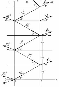
I II III

Fig.5 The schematic picture of the multiple 2D reflections, over-barrier penetrations and transmissions of non-relativistic particles.

In the case k=, when q=0 (see Fig.5) i.е. the incident plane wave is perpendicular to the first boundary of interface and Dy=0, it is not difficult to see that =1 and , due to the conservation of the flux in the first transmission through points (x=y=0) and (x=0, y=a). In the case of 1-D penetration (at q =0, when the incident plane wave is perpendicular to the first boundary of interface and Dy=0) all expressions, including the last expressions n=1,2,…, in (20)-(24) are coincident with the correspondent 1-D expressions in [37], represented with the help of the time analysis (for the stationary phase) to the 1-D tunneling.

Now let analyze sub-barrier tunneling at E_x<V₀. If the angle q is sufficiently large (, where is defined by eq. =V₀), then < V₀ and the values of are imaginary, i.е. = ic with c >0 and there is sub-barrier tunneling, . In this case, instead of over-barrier penetration, for description sub-barrier tunneling it is necessary introduce c instead of with the help of substitution =ic. And instead of current (in II) waves , the evanescent a_n and anti-evanescent wavesb_nexp(gx) will appear. The correspondent picture is represented in Fig.6.

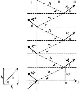
Fig.6.The schematic description of the multiple 2-D reflections, sub-burrier penetrations and transmissions of a non-relativistic particle.

In this case factually utilized the analytic continuation from the region of real (over-barrier) wave numbers to the region of imaginary (under-barrier) wave numbers similarly to that was made in [37]. The obtained results, like to (20)-(24) but with substitutions ® ic, ®, ® coincide with the correspondent 1-D results in [37].

Instead of the shift Dy along the axis y, defined for the above-barrier transmission by equations (19a) and (19b) and depicted in Fig.5, it is necessary to use the expressions, like (19b):

D_n y=(, (19с)

where

= (n=1,2,…), (25)

and

(n=1,2,…). (26)

The quantities и represent the phase times of motion (i.е. the times of moving for a quasi-monochromatic particle in the approximation of the stationary phase) for the n-th step at the under-barrier tunneling through point x=a and the n-th step at the external reflection from the first barrier in point x=0, respectively ([8]). Of course, the shifts D_ny with different values of n=1,2,3,… are different (due to the not large numerical increase of and for increasing numbers n, but they are always proportional to 2/vc in the limit ca ® ¥). Tunneled and externally reflected waves of the increasing order with the increasing of number n are quickly damped due to the factor exp(–ca) in expressions for and, and finally vanish.

In [39] without the strict theoretic justification and neglecting the multiple internal reflections and transmissions (instead of analytic continuation, used in [33-37]) there was used only one usual linear combination of waves for the k_x – component inside the region II and only one wave for k_y –component inside the region II, and there was obtained the following expression for only one shift along axis y in the second boundary of interface (between II and III)

Dy =( (19d)

which is represented in Fig.7, when

=t_tun=a/v+h¶argA_T/¶E=(vc)^-1 for ca®¥ (27)

with A_T=,, , , and in the result there was obtained only one transmitted (in III region) 2-D wave which is moving in the parallel direction to the incident wave.

Thus, we have confronted two approaches for 2-D sub-barrier tunneling for the sub-barrier tunneling of a particle. The first one is represented in Fig. 6 with the infinite series of internal reflections and transmitted waves – with the help of formulas (20)-(24), with changing ® ic, ®, ® and with the help of shifts (19c,d). The second one is represented in Fig.7 with the only one shift during tunneling and the оnly one transmitted wave, which is moving in parallel to the incident wave, in total neglecting by the multiple internal reflections and the correspondent transmitted waves.

Fig.7. The scheme of 2-D tunneling with one reflected and one transmitted wave.

Both approaches indicate to the non-local behavior of the sub-barrier tunneling which brings to the Hartmann phenomenon for the phase tunneling time in the limit ca ® ¥. This phenomenon consists in the independence of the phase tunneling time on the barrier width ([8]). And it remains only to confirm what from approaches really describes the sub-barrier tunneling. Till now our approach is confirmed (Fig.6) by several methods, described in [38], and preliminary is verified by rather old (however without the real data processing) experimental observations, published in [40-41].

2-D penetration and tunneling of a photon through the barrier. With taking into account the similarity of the photon and particle motion we can extend the obtained results on the photon 2-D penetrations and tunneling. Fig.5-7 can be also used for photons, propagating in the homogeneous glass medium I and III, penetrating or tunneling through the homogeneous air layer. In this case the quantity

(28)

is the refraction light coefficient in the glass (if one suppose that the refraction light coefficient in air is 1), and in Fig.6 it is described the penetration of photons through the layer II for the angles lesser the critical angle , i.е. than the angle of the total internal reflection for incident photons, polarized perpendicularly to the plane x-y of the light incidence.

Fig.6 and 7 describe the violated total internal reflection of the polarized light, tunneling through the slab II, for the incidence angle (violated in the sense of the partial transmission through the layer II in the glass medium III) in both approaches, using 2-D tunneling for particles with the multiple internal reflections, represented here (and also in some different form for the light in [40-41]) (Fig.6), or using the description of the 2-D tunneling of the non-relativistic particle and photon, represented in [39] (Fig.7). We hope that the correct final refined optical experiments can give the clear demonstration of the multiple internal reflections and multiple transmitted waves, as it was previously analyzed in [40-41].

VI. The 3-D tunneling. One can enter upon such problem in a simple way, naturally extending the 2-D problem of tunneling (for axes х and у) in the 3-D one(in axes х, у and z) and supposing the surfaces of the interface to be 2-D (parallel to the plane of axes у and z) with the previous direction of tunneling along the axis х. Leaving this problem to the opinion of readers, we can also pass to the spherically symmetrical tunneling problem, where the main role is placed to the radial coordinate. Such problem is usually exposed not only in many monographs on quantum mechanics, but even in almost all contemporary articles on nuclear physics in the limits of WKB-approximation. Only in [42] this 3-D spherically symmetric problem had been exposed in the limits of the self-consistent quantum mechanics.

VII. Summary and further perspectives.

1) So, here there was studied, basing on similarity of particle and photon tunneling, the theoretic results of 2-D and 3-D photon tunneling and multiple internal reflections. Then there are proposed the refined optical experiments for these phenomena in the continuation of [40-41].

2) There is remained an interesting perspective to resolve the problem of the signal superluminality of the modulated waves in the electromagnetic (photon) tunneling in addition to the resolved group-velocity superluminality in the photon tunneling.

References

1.A.I.Akhiezer, V.B. Berestezki, Quantum Electrodynamics, FM, Moscow, 1959 [in Russian].

2. S.Schweber, An Introduction to Relativistic Quantum Field Theory, Row, Peterson &Co,Evanston, Ill, 1961 (chapter 5.3).

3. A.Enders, G.Nimtz, J.Phys.I (France) 2 (1992)1693; J.Phys.I (France) 3 (1993)1089; Phys.Rev. B 47 (1993)9605; Phys.Rev. E 48(1993)632; G.Nimtz, in: Tunneling and ist Applications, World Sci., Singapore, 1997, pp.223-237.

4. J.D.Jackson, Classical Electrodynamics, Wiley, N.Y.,1975, section 8.3.

5. P.M.Morse, H.Feshbach, Methods of Theoretical Physics,McGraw-Hill, N.Y.,1953 part II (chapter 13).

6. L. Brillouin, Wave Propagation and Group Velocity, Academic Press, N.Y., 1960.

7. J.Jakiel, V.S.Olkhovsky, E.Recami, Phys.Lett.A 248 (1998)156-160.

8. V.S.Olkhovsky, E.Recami, Phys.Rep. 214 (1992)339; V.S.Olkhovsky, E.Recami,J.Jakiel, Phys.Rep.398 (2004)133.

9. L.B.Felsen, N.Marcuvitz, Radiation and Scattering of Waves,v.1, Prentice-Hall, N.Y.,1973 (chapter1.5).

10. M.Abolhasani, M.Golshani, Phys.Rev., A62 (2000) 012106.

11. V.S.Olkhovsky,E.Recami,F.Racity,A.K.Zaichenko,J.Phys. (France)5 (1995)1351.

12. E.Wigner, Phys.Rev. 98 (1955)145.

13. T.E.Hartmann, J.Appl.Phys.33 (1962)3427.

14. J.Ch.Bose, Bose Institute Transactions, 42 (1927).

15 A.M.Steinberg, P.G.Kwiat, R.Y.Chiao, Phys.Rev.Lett. 71 (1993)708; R.Y.Chiao, P.G.Kwiat, A.M.Steinberg, Scient.Am., 269:2 (1993)38.

16. Ch.Spielman, R.Szipoecs, A.Stingl,F.Krausz, Phys.Rev.Lett. 73 (1994)2308.

17. Ph.Balcou,L.Dutriaux, Phys.Rev.Lett. 78(1997)851.

18. V.Laude,P.Tournois, J.Opt.Soc.Am. B16 (1999)194.

19. A.Haibel,G.Nimtz, A.A.Stahlhofen,Phys.Rev.E63 (2001)047601.

20. V.S.Olkhovsky, E.Recami, G.Salesi,Europhys.Lett. 57 (2002)879.

21. V.S.Olkhovsky, E.Recami, A.K.Zaichenko, Europhys.Lett. 70(2005)712.

22. G.Nimtz,A.Enders, H.Spieker, J.Phys.I (France) 4 (1994)565.

23. S.Longhi,P.Laporta, M.Delmonte, E.Recami, Phys.Rev. E65 (2002) 046610.

24. R.Bonifaccio(ed.), Mysteries,Puzzles and Paradoxes in Quantum Mechanics, AIP,Woodbury, N.Y., 1999, R.Y.Chiao –pp.3-13; G.Nimtz –pp.14-31;E.Recami- pp.32-35; A.Steinberg- pp.36-46.

25. D. Mugnai, A.Ranfagni, L.S.Schulman (eds.),Time’s Arrows, Quantum Measurement and Superluminal Behavoir, Napoli, Italy, Oct.3-5,2000 (C0nsiglio Nazionale delle Ricerche,Roma), E.Recami-pp.17-36;G.Nimtz,A.Haibel,R.- M. Vetter- pp.125-138; V.S.Olkhovsky- pp. 173-178.

26. G.Nimtz, Progress in Quantum Electronics,27 (2003)417-450.

27. H.G.Winful, Phys.Rep. 436 (2006)1.

28. E.Recami, J.Phys.:Conf.Series 196;1 (2009) 012020.

29. G.Nimtz, Found.Phys.39:12(2009)1346-1355.

30. A.B.Shvartsburg, G.Petite, M.Zuev, J.Opt.Soc.Am.,B28(2011)2271-2276.

31. A.Aharonov, N.Erez,M.Reznik, Phys.Rev. A65 (2002)052124.

32. F.Cardone, R.Mignani, V.S.Olkhovsky, Phys.Lett.,289 (2001)279; Mod.Phys.Lett.,14 (2000)109;J.Phys.I (France),7 (1997)1211.

33. J.H.Fermor, Am.J.Phys.,34 (1966)168.

34.R.W.McVoy,L.Heller and M.Bolsterli, Rev.Mod.Phys.,39 (1967)245.

35. A.Anderson, Am.J.Phys.,57 (1989)230.

36. S.P.Maydanyk, V.S.Olkhovsky, A.K.Zaichenko, J.Phys.Studies (Ukraine), 6 (2002)24.

37. F.Cardone, S.P.Maydanyk, R.Mignani, V.S.Olkhovsky, Found.Phys. Lett., 19:5(2006)441.

38. V.S.Olkhovsky, M.V.Romanyk, J.Mod.Phys.,2:10 (2011)1166-1171, doi:110,4236/jmp.2011.210145.

39. A.M.Steinbergand R.Y.Chiao, Phys.Rev.,A49 (1994) 3283.

40. C.K.Carniglia and L.Mandel, J.Opt.Soc.Am.,61 (1971) 1035.

41. S.Zhu, A.W.Yu, D.Hawley and R.Roy, Am.J.Phys.,54 (1986)601.

42. V.S.Olkhovsky, V.Petrillo, J.Jakiel, W.Kantor, Central Eur. J. Phys.,6 (1) (2008)122 ; V.S.Olkhovsky, M.V.Romanyuk, Nuclear Physics and Atomic Energy (Ukraine, Kiev),10, N3 (2009)273.