On the Question of an Unsearched Algorithm

to Identify the Adaptive Model

Introduction

The paper deals with the parametric identification, using unsearched identification algorithm with adaptive model (UIAAM) [1]. The algorithm uses the idea of setting a minimum of the difference (residual) outputs of a real object and model, excited by the same input signal [2]. The unsearched algorithms are oriented to function in real time. Existing UIAAM are designed for parameter identification.

UIAAM in the state space is characterized that the process which is identified, the adaptive model and algorithm of its settings are described in the state space, and the observed (output) variables are functions of the state vectors.

With regard to UIAAM, in the description of the process and the model we will limit by the function of the observed value of x, u, t

,

where is identified parameter of the process.

In general, the characteristics of a custom model and the conditions of its observation are regarded as different from the characteristics of the object and functions of its observations, i.e. .

We are forming some residual vector:

The task of the UIAAM is to provide the norm of the error vector and the norm of the difference parameters in a specified sufficiently small area.

The UIAAM function can be achieved by tuning the algorithm model of the form: .

The block diagram corresponding to the expressions is shown in Figure 1.

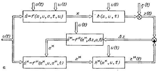
Fig. 1. Block diagram of the algorithm

UIAAM for continuous object as described in the state space

Let us consider the case of linear object and the model of the first order.

The linear and the linear model are been describing in the state space as follows:

(1)

We consider the differences: , , .

All vectors are considered directly observed (measured).

Subtracting the second equation of (1) from the first, we find:

. (2)

Add and subtract to the right side of equation (2):

,

then

. (3)

In (3) match the current configuration model and they are known, is directly determined from the measured values, as well as . Thus, the signal observed discrepancy may be taken as:

To ensure the sustainability of the system, we use the Lyapunov’s function. The Lyapunov’s function is sought in the form of the positive-definite quadratic form:

where are the positive-definite diagonal matrixes of predetermined coefficients.

We have

Let the values be

(4)

then

Expression (4) is transformed to

. (5)

This algorithm cannot be accurately tuned to implementation to the model, as both andare not exactly known. However, at relatively slow change and or sufficiently large gain coefficients, the members , can be ignored and we can replace (5) by the algorithm

This algorithm is implemented by setting up the model. We write it in matrix form, thinking that , do not depend on i

In accordance with the criterion of the Lyapunov’s stability, this system will be stable at the origin. Finally we have

(6)

An example of the use of the technique

There is the set A = [-1, 1, -2 -3]. We have to provide the identification of the parameters A, using the method UIAAM . We gather the scheme of the original system model (Fig. 2) and the identifier (Fig. 3), according to the equations (6).

The matrix B is assumed to be [1, 1]. The adjustment coefficient k we define as [100 0, 0100]. The initial conditions of the integrator in the loop identifier are equal to the initial value of the parameter A.

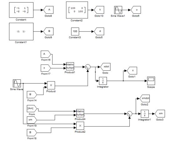
Fig. 2. The initial system and its model in the Simulink environment

Fig. 3. Identifier of the system in the Simulink environment

The outputs of the identifier and the signals of the parameter A is presented in Fig. 4.

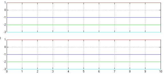
Fig. 4. The outputs of the identifier and the signals of the parameter A

Based on the results presented in Fig. 4, we verify the effectiveness and efficiency of the considered method of identification.

References

1. Krasovskij A.A. Handbook of the theory of automatic control. – M.: Nauka, 1987. – 712 p.

2. Karabutov N.N. Adaptive identification of a system. – M.: KomKniga, 2006. – 384 p.