Agnieszka
Poczta-Wajda, PhD
The Poznań
University of Economics
Department of
Macroeconomics and Agricultural Economics
COMPETITIVENESS OF AGRICULTURAL PRODUCTS FROM
WELL-DEVELOPED COUNTRIES ON WORLD MARKETS IN THE LIGHT OF DIFFERENT
LIBERALIZATION SCENARIOS
Introduction
Competitiveness
is a process in which producers try to present an offer better than the others
in order to encourage a buyer to chose their product [Iwan 2006]. A product is
said to be competitive when it is better that the alternative one in regard to
a specific criterion, i.e. price, quality or another feature. Agricultural
products are considered to be an example of very homogenous goods, so price is
very often a criterion which decides about their competitiveness. Agricultural
products from developing countries are usually cheaper than those produced in
developed countries mainly because developing countries enjoy some comparative
advantages like better natural conditions and cheaper labour. Market share
measures a competitive position of a good [Kasprzyk 2006]. Agricultural
products from developing countries should therefore be more price competitive
than the similar products from developed countries and possess significant
share in world agricultural export. But this is not the case.
In the beginning of 60’s, share of
developed countries in world agricultural import accounted for 60% and in world
agricultural export for 50%. By the middle of 80’s, these values changed a lot
and a share of developed countries in world agricultural import declined to 40%
and share in world agricultural export raised to 70%. What is more, this
process is still progressing [Tyers 1992, WTO Database]. It is happening
because of the very protective agricultural policy of developed countries
(especially EU, US and Japan). Measures of market access, export subsidies and
domestic financial support cause that producers from developing countries find
it difficult to sell their products on the markets of developed countries,
whereas producers from developed countries are able to sell their products on
the world markets at a very cheap prices. Consequences of this situation are
especially adverse for the least developed countries, in which trade with
agricultural product (non-processed) has a crucial meaning for their economy
and employment. Financial support for the farmers from developed countries
influences the prices on world markets and reduce them under the level of
profitability in many developing countries [Koo, Kennedy 2006]. This problem
has been recognized on the international arena and the World Trade Organization
(WTO) leads constant negotiations which aim to liberalize international trade
with agricultural products. This process seems to be extremely difficult
because of the protests of farmers’ lobbies from developed countries. On the
one hand, farmers are afraid of competition exacerbation on domestic markets,
and on the other hand, they do not want to lose their own competitiveness on
the world markets [Kosewska, Kalicki 2008].
The aim of this paper is to
indicate how chosen measures of trade policy (tariffs and export subsidies)
from developed countries influence prices on internal and external agricultural
markets and the same determine competitive position of producer. Further, author of
this paper is going to analyze the effects of future potential liberalization
of agricultural trade under the WTO on the competitiveness of agricultural
products from developed countries. The partial equilibrium model of
agricultural sector AGLINK will be used to evaluate different liberalization
scenarios.
Impact of intervention trade policy of developed
countries on the competitiveness of agricultural products
A country which
share of world trade flows is big enough that it can influence world markets
and the equilibrium price is called to be a “big” one from the economic point
of view [Świerkocki 2004]. Well-developed countries, because of their
share in world agricultural trade, are “big” countries and that is why the
measures of intervention used in well-developed countries influence also prices
on the world markets. Figure 1 illustrates economics consequences of export
subsidy in a country A, which is a “big” country, and its impact on the world
market price.
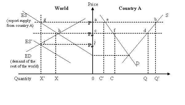
Figure 1. Economic consequences of a „big” country interference in export price
level
Source: R. Tyers, K. Anderson, Disarray in
World Food Markets. A Quantitative Assessment. Cambridge University Press,
Cambridge 1992, p. 129.
In the base
situation, price on world market amounts Pw. Country A decides to
support export, introduces export subsidy and the same rises domestic price
from Pw to P. Amount of export increases from CQ (=0X) to C’Q’
(=0X’). At the same time, additional amount of export from country A on the
world market lowers the world prices to the level Pw’. Country A must
extend the value of subsidy to Pw’P. Of course the winners are
producers from country A, who can sell more at higher price (area abdc), however consumers from this
country lose (area aefc). Difference
between producers’ advantages and consumers’ disadvantages represents area ebdf (or area gach). One must also remember to consider taxpayer lose (area gaij). Total net effect for the country A welfare is negative. A part of this
lost will be compensated on the world market by the gains of foreign importers
(area jhci), however the world net
welfare will also decline (area ghj).
The conclusion is that a “big” country, which rises the price of good over the
world level, loses more than a “small” country in the similar situation and the
lost of world net welfare is also bigger [Koo, Kennedy 2006].
Figure
2 illustrates economics consequences of tariff in a country A, which is a “big”
country, and its impact on the world market price.
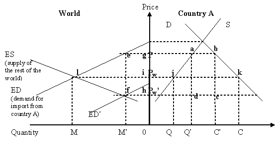
Figure 2. Economic consequences of a „big”
country interference in import price level
Source:
R. Tyers, K. Anderson, Disarray in World Food Markets. A Quantitative
Assessment. Cambridge University Press, Cambridge 1992, p. 131.
Country A decides to protect domestic producers from the foreign
competition and introduces a tariff. Domestic price increases from world level Pw to level P. Amount
of production in country A rises from 0Q to 0Q’ and amount of consumption falls from
QC (=0M) to Q’C’ (=0M’). Lower import demand in country A causes decline of
world price to level Pw’. In order to keep domestic price at level
P, country A must introduce a higher tariff Pw’P. Area abcd (or eghf) represents the value of tariffs coming into country A budget.
Producers’ gains are equal to area gaji,
whereas consumers’ loses are illustrated by area igbk. Net welfare effect will depend from the relation between area
jabk and area abcd. This relation will in turn depend from the elasticity of
demand for the import from country A (the lower elasticity, the bigger lost)
and the elasticity of supply of the rest of the world (the higher elasticity,
the bigger lost). However it is worth mentioning, that the effect for the world
net welfare will be negative (area efl)
and the effect for the rest of the world net welfare will also be adverse (area
hfli).
Presented examples of
economic consequences of tariff and export subsidy introduction in a “big”
country show how well-developed countries influence competitive situation on
the world markets. They do not only support domestic producers and let them
gain higher prices, but also decrease prices on world markets which reduce the
profitability of production in the other countries. Decline of prices on the
world markets is not harmful for producers from well-developed countries,
because it is being compensated with subsidies or higher domestic prices. One
can find this situation on many agricultural markets. Liberalization of trade
with agricultural goods under the WTO (reduction of tariffs and withdrawal of
export subsidies) should therefore result in increase of prices on the world
agricultural markets and decline in well-developed countries share in
agricultural export. Price competitiveness of products from well-developed
countries should decline towards products from developing countries, which use
comparative advantages (cheaper means of production).
Scenarios of
agricultural trade liberalization on the chosen agricultural market with the
use of AGLINK model
Agricultural trade
liberalization, as presented above, could lead to lost of price competitiveness
of supported agricultural products from well-developed countries. Because
results of Doha Round are still very dubious, agricultural economists try to
predict effects of different scenarios of WTO negotiations on agriculture.
Global economic models of equilibrium might be very useful in such analysis.
With the use of these models one can survey quantitative relations between the
whole economies, as well as single sectors and economies [van Togeren, van
Meijl, Surry 2001]. Usually we distinguish two types of global economic models:
general equilibrium models (cover the whole economies) and partial equilibrium
models (cover only one sector).
In this survey, a partial equilibrium
model AGLINK-Cosimo was used. Module AGLINK is a dynamic, recursive,
demand-supply partial equilibrium model of agricultural sector in OECD member
countries and aggregate of the rest of the world. It was presented for the
first time in 1992 by the OECD and was used for mid-term prognosis of changes
in agricultural market variables in 10 member countries/groups caused by the
shifts in agricultural policy. It was then completed with four non-member[1]
countries, which had an important meaning in world trade with agricultural
goods and in 2004 it was combined with FAO Cosimo module, which included other
non-OECD countries. Because AGLINK is a partial equilibrium model it embraces
only chosen agricultural markets[2].
It is assumed that other sectors do not influence the agricultural sector,
unless they are included in demand or supply equations as exogenous variables
(i.e. macroeconomic data)
[Thompson,
Smith, Elasri 2007]. Variables in model include annual values of supply,
consumption, stocks, trade flows, prices[3]
and measures of trade policy (tariffs, tariff rate quotas, export subsidies)
and domestic support policy, which vary in every country[4].
Version 2006 of the model includes 10 800 equations and more than
30 000 variables from 39 countries and 16 regions.
One of the applications of the model is
the possibility to produce mid-term forecasts of market variables changes as a
result of different scenarios of agricultural and trade policy reforms. OECD,
each year, publishes a base simulation in which it is assumed that agricultural
policies in countries included in the model and macroeconomic conditions will
not change. Analysis of any eventual changes in agricultural policy should be
done with reference to the OECD base simulation. To run own simulation one must
shock some exogenous variables in the model and then compare results with the
original ones.
Simulations in this paper are based on
five different scenarios of WTO agricultural negotiations results. In all
scenarios it is assumed that only measures of market access (tariffs and tariff
rate quotas) and export subsidies are going to liberalized. Possible changes in domestic support policy
are deliberately neglected. These scenarios are based on following assumption:
·
scenario A –
full multilateral elimination of export subsidies in equal rates in the years
2009-2013. It as a scenario of very “gentle” liberalization and quite possible,
because during the Hong Kong Ministerial Conference member countries of WTO
have already agreed for the elimination of export subsidies until 2013,
·
scenario B –
full multilateral elimination of export subsides and full multilateral
reduction of tariffs in equal rates in the years 2009-2013. It as a scenario of
very “strict” liberalization and rather not possible,
·
scenarios C,
D and E - full multilateral elimination of export subsides and tariff reduction
based on modified proposals of US, EU and G-20 presented in the so called July
Package (table 1).
Table 1. Tariff reduction scenarios based on proposals of US, EU and G-20
in July Package
|
Tariff
base level |
Tariff reduction (in %) |
||
|
Scenario C (US proposal) |
Scenario D (EU proposal) |
Scenario E (G-20 proposal) |
|
|
> 120% 60%-120% 20%-60% 0%-20% |
85 75 65 55 |
60 50 45 35 |
75 65 55 45 |
Source: Own elaboration based on WTO member countries proposals from WTO
web page www.wto.org.
Scenarios
B, C, D and E do not consider issue of sensible products, because countries did
not present a list of such products. As far as tariff rate quotas are concerned,
50% increase of quota with lower tariff is assumed[5].
These scenarios also assume liberalization of agricultural trade in Russia
because of a very possible accession of Russia to WTO. Generally, scenario A
modifies 9 exogenous variables and scenarios B, C, D and E modify 114 exogenous
variables. Results of AGLINK simulations based on this five scenarios are
presented in table 2. Because of the size of the model and number of variables,
only chosen countries and most important markets are going to be discussed.
On the majority of the markets,
liberalization would lead to increase of prices over the base simulation,
however the intensity of this process would be dependant on the single scenario
assumption. Only prices for wheat, oil seeds and pork would behave differently
and fall under the price level in base simulation. It is probably because
protection measures on these markets are already relatively week and export of
this goods from well-developed countries is not supported. However one needs to
remember that price changes caused by export subsidies elimination and tariff
reduction are not the only factors which can influence size of production and
trade flows on given market. In many cases, agricultural markets are strongly
dependant on domestic support policy, which is not analyzed in the scenarios.
Nevertheless, on some markets reduction in trade policy measures would be
enough to get some crucial adjustments of production and trade flows. Above
statement concerns especially beef market. On beef world market, liberalization
would lead to a small production increase and an essential increase in trade
flows. The biggest growth (30%) in beef export in world scale would occur in
scenario B, in which all export subsidies and tariff are eliminated. Scenario
D, the one proposed by EU, would lead only to 17% growth in beef world export.
In scenario A, in which only export subsidies are eliminated, export of beef on
the world market would probably even fall below base simulation. This could be
a result of a strong decline in beef export from EU. In this scenario, import
of beef in EU would also decline because of emerge of excess supply, which
could not be exported without subsidies. Reduction of very high tariffs for
beef in EU (scenario B, C, D and E) would in turn lead to a very strong import
increase (from 150% do even 270% dependant from scenario) and almost full
reduction of beef export. Very expensive beef from EU could not manage
competition on world market.
Table 2. Impact of different liberalization scenarios on chosen
agricultural markets (results for the year 2014)
|
US |
Wheat |
Rice |
Pork |
Beef |
SMP |
Butter |
|
|
Production (000 t) |
Base simulation |
61085,2 |
8209,7 |
9757,7 |
12786,1 |
545,6 |
657,9 |
|
Relative change to base simulation (%) |
Scenario A |
-0,2 |
0,0 |
-0,2 |
0,0 |
-1,4 |
-1,3 |
|
Scenario B |
-0,4 |
0,1 |
-0,3 |
0,7 |
-1,3 |
-1,2 |
|
|
Scenario C |
-0,3 |
0,1 |
-0,4 |
0,5 |
-1,3 |
-1,2 |
|
|
Scenario D |
-0,3 |
0,1 |
-0,3 |
0,4 |
-1,4 |
-1,3 |
|
|
Scenario E |
-0,3 |
0,1 |
-0,3 |
0,4 |
-1,3 |
-1,2 |
|
|
Export (000 t) |
Base simulation |
29244,7 |
4067,3 |
1341,4 |
1284,7 |
165,6 |
20,0 |
|
Relative change to base simulation (%) |
Scenario A |
-1,1 |
0,0 |
-1,1 |
-0,4 |
-4,2 |
-100,0 |
|
Scenario B |
-2,8 |
0,3 |
-8,3 |
0,5 |
-6,1 |
-100,0 |
|
|
Scenario C |
-2,5 |
0,3 |
-7,1 |
47,7 |
-5,9 |
-100,0 |
|
|
Scenario D |
-2,2 |
0,2 |
-5,3 |
43,5 |
-5,4 |
-100,0 |
|
|
Scenario E |
-2,4 |
0,3 |
-6,4 |
45,7 |
-5,7 |
-100,0 |
|
|
Import (000 t) |
Base simulation |
3116,6 |
522,2 |
970,9 |
1923,3 |
1,0 |
18,8 |
|
Relative change to base simulation (%) |
Scenario A |
0,0 |
0,0 |
-0,5 |
0,0 |
0,0 |
0,0 |
|
Scenario B |
0,0 |
0,0 |
-1,4 |
23,6 |
0,0 |
0,0 |
|
|
Scenario C |
0,0 |
0,0 |
-1,4 |
23,1 |
0,0 |
0,0 |
|
|
Scenario D |
0,0 |
0,0 |
-1,1 |
23,0 |
0,0 |
0,0 |
|
|
Scenario E |
0,0 |
0,0 |
-1,3 |
23,0 |
0,0 |
0,0 |
|
|
EU |
Wheat |
Rice |
Pork |
Beef |
SMP |
Butter |
|
|
Production (000 t) |
Base simulation |
133220,9 |
1690,8 |
22370,1 |
7641,7 |
899,8 |
1897,2 |
|
Relative change to base simulation (%) |
Scenario A |
0,8 |
0,0 |
0,2 |
-0,3 |
-4,5 |
-1,7 |
|
Scenario B |
2,2 |
0,0 |
-6,0 |
-10,8 |
-8,9 |
-2,8 |
|
|
Scenario C |
1,9 |
0,0 |
-5,1 |
-9,2 |
-8,3 |
-2,6 |
|
|
Scenario D |
1,6 |
0,0 |
-3,6 |
-6,6 |
-7,3 |
-2,4 |
|
|
Scenario E |
1,8 |
0,0 |
-4,5 |
-8,1 |
-7,9 |
-2,5 |
|
|
Export (000 t) |
Base simulation |
15212,1 |
246,8 |
1445,3 |
200,6 |
105,3 |
184,6 |
|
Relative change to base simulation (%) |
Scenario A |
19,8 |
0,0 |
3,0 |
-59,8 |
-23,5 |
-41,6 |
|
Scenario B |
57,3 |
0,0 |
18,2 |
-100,0 |
-8,1 |
-48,9 |
|
|
Scenario C |
51,3 |
0,0 |
16,0 |
-100,0 |
-10,4 |
-48,2 |
|
|
Scenario D |
41,7 |
0,0 |
12,4 |
-100,0 |
-14,3 |
-46,7 |
|
|
Scenario E |
47,4 |
0,0 |
14,6 |
-100,0 |
-12,0 |
-47,7 |
|
|
Import (000 t) |
Base simulation |
6517,3 |
1268,5 |
32,0 |
723,0 |
9,3 |
79,0 |
|
Relative change to base simulation (%) |
Scenario A |
0,0 |
-0,1 |
0,0 |
-11,2 |
0,0 |
0,0 |
|
Scenario B |
0,0 |
-0,3 |
0,0 |
269,4 |
0,0 |
0,0 |
|
|
Scenario C |
0,0 |
-0,1 |
0,0 |
223,9 |
0,0 |
0,0 |
|
|
Scenario D |
0,0 |
-0,2 |
0,0 |
151,7 |
0,0 |
0,0 |
|
|
Scenario E |
0,0 |
-0,2 |
0,0 |
194,5 |
0,0 |
0,0 |
|
|
WORLD |
Wheat |
Rice |
Pork |
Beef |
SMP |
Butter |
|
|
Production (000 t) |
Base simulation |
689776,9 |
484211,7 |
121327,8 |
76506,9 |
3405,4 |
9773,3 |
|
Relative change to base simulation (%) |
Scenario A |
-0,1 |
0,0 |
0,0 |
0,1 |
-1,0 |
-0,5 |
|
Scenario B |
-0,5 |
-0,2 |
-1,1 |
1,3 |
-2,2 |
-1,9 |
|
|
Scenario C |
-0,5 |
-0,2 |
-0,9 |
1,0 |
-2,1 |
-2,1 |
|
|
Scenario D |
-0,4 |
-0,1 |
-0,7 |
0,6 |
-1,8 |
-1,5 |
|
|
Scenario E |
-0,4 |
-0,1 |
-0,8 |
0,8 |
-2,0 |
-1,9 |
|
|
Export (000 t) |
Base simulation |
125463,3 |
33652,2 |
6811,6 |
10072,9 |
1050,7 |
794,3 |
|
Relative change to base simulation (%) |
Scenario A |
0,7 |
0,0 |
0,1 |
-0,8 |
-1,4 |
-6,3 |
|
Scenario B |
3,2 |
1,0 |
5,8 |
30,0 |
-0,9 |
-6,4 |
|
|
Scenario C |
2,8 |
0,9 |
5,0 |
24,1 |
-1,1 |
-6,4 |
|
|
Scenario D |
2,2 |
0,8 |
4,3 |
17,6 |
-1,2 |
-6,4 |
|
|
Scenario E |
2,5 |
0,8 |
4,7 |
21,3 |
-1,2 |
-6,4 |
|
Source: Own estimations based on
AGLINK model.
Such a
strong increase in beef import in EU would probably resulted from lower beef
production and higher beef consumption caused by low beef prices. In many
well-developed countries, cheaper beef would substitute pork consumption and
production (US and EU). Liberalization would also lead to decline in export of
dairy products from EU, which are presently supported with a very high export
subsidies.
It is worth mentioning, that in
different liberalization scenarios, export of wheat from EU would increase.
This phenomenon can by explained by the wheat tariff reduction in developing
countries[6]
and higher wheat demand (for the feeds) on the world markets. Simulation results
show that the wheat price would fall below the base simulation level. It would
lead to decline in production in less developed countries. However, farmers in
EU are supported with domestic policy measures (direct payments), which could
sooth adverse effects of wheat price decline. In US one can expect essential
changes on beef, dairy and pork markets. Adjustments on crop markets would be
rather moderate, because crop producers in US are also protected by domestic
support programs and trade measures have narrow meaning for them.
Conclusions
Agricultural policy
of well-developed countries, because of their economic size, supports not only
domestic farmers but also destabilizes world agricultural markets. Tariffs,
export subsidies and domestic support measures lead to decline of agricultural
prices on world markets under the level of profitability for many developing
countries. Simultaneously, high financial support for farmers from
well-developed countries allow them to compete and to win this competition both
on domestic and world markets. Agricultural trade liberalization, to which
tends WTO, could reduce price competitiveness of products from well-developed
countries.
Simulations with partial equilibrium
model AGLINK show that elimination of export subsidies and reduction of tariffs
would lead to stronger effects on meet markets than on crop markets. Special
meaning for the developing countries would have liberalization on the beef and
dairy market. Simulation results also indicate that on the majority of
agricultural markets in well-developed countries effects of export subsidies and tariff reduction would
be rather weak. Farmers in these countries are after all supported with wide
system of domestic policy measures. Additional, there exist a high probability,
that eliminated subsidies and tariffs would be substituted with another form of
support, which would compensate potential loses for farmers. One can conclude,
that only liberalization of agricultural trade policy combined with
liberalization of domestic support could lead to any essential shifts in the
structure of international trade with agricultural products.
Summary
This paper considers some issues of the
developed countries agricultural policy impact on the world agricultural
markets. On the example of tariffs and export subsidies it was shown that these
measures increase price competitiveness of the products from developed
countries. Further, the partial equilibrium model AGLINK was used to evaluate
potential consequences of agricultural trade liberalization under the WTO. It
was proved that the biggest decline of competitiveness of agricultural products
from developed countries would occur on the beef and dairy market.
Bibliography:
Iwan B.
(2006): Konkurencyjność polskich produktów mleczarskich na
rynku Unii Europejskiej, [in:] Agrobiznes 2006. Konkurencja w agrobiznesie –
jej uwarunkowania i następstwa, ed. S Urban, Wydawnictwo AE we
Wrocławiu, Wrocław, p. 321-328.
Kasprzyk A.
(2006): Konkurencyjność wybranych przedsiębiorstw przemysłu
mięsnego w opinii konsumentów, [in:] Agrobiznes 2006. Konkurencja w
agrobiznesie – jej uwarunkowania i następstwa, ed. S Urban, Wydawnictwo AE
we Wrocławiu, Wrocław, p. 386-392.
Kosewska M.,
Kalicki A. (2008): Analiza stanu rokowań w ramach Światowej
Organizacji Handlu (WTO) – tzw. Runda z Doha, FAPA FAMMU, Warszawa, p. 18.
Koo W.,
Kennedy P. (2006): The Impact of Agricultural Subsidies on Global Welfare,
“American Journal of Agricultural Economics”, nr 88(5), p. 1219-1226.
Świerkocki J. (2004): Zarys międzynarodowych
stosunków gospodarczych. PWE, Warszawa, p. 133.
Thompson W., Smith G., Elasri A. (2007): The Medium-Term Impacts
of Trade Liberalization in OECD Countries on the Food Security of Nonmember
Economies. [in:] Reforming Agricultural
Trade for Developing Countries, ed. A. McCalla, J. Nash, The World Bank,
Washington DC, p. 183.
van
Tongeren F., van Meijl H., Surry I. (2001): Global models applied to
agricultural and trade policies: a review and assessment, “Agricultural Economics”,
nr 26, p. 150.
Tyers
R., Anderson K. (1992): Disarray in World Food Markets. A Quantitative
Assessment. Cambridge University Press, Cambridge, p. 21.
WTO Database, www.wto.org