Shapovalova O., Gnuchуkh L., Hozyaenova J.

Kharkov National University of civil engineering and architecture, Ukraine

Modeling the dynamics of the currency rate

For Ukraine, which undergoes the economic reforms, the issue of forecasting developments in the foreign exchange market is particularly important both at the macro and at micro levels. Almost every citizen of the country observes the exchange rates. Current values and leading national currencies are the first things which are reported about in any economic sector of the news today. The stabilization of exchange rates has become one of the main topics during the discussion of issues related to the global economy in international negotiations.

When forecasting such integrated indicators as exchange rate, economics identifies two basic set of methods: fundamental and technical analysis. Fundamental analysis involves the examination of trends in pricing, based on the basic factors of the economy, which include, in particular, interest rates, taxes, unemployment, state budget, inflation, the stability of the political system and so on. The basis of technical analysis is the fact that the behavior of prices has already taken into account all the existing factors. In general terms, technical analysis expects the accumulation of real history of price changes and conclusions’ building concerning likely future trend. Thus, the sequence of time-ordered data forms a time series.

Works of N.D. Kondrateva, Schumpeter, Dzh.M. Keyns, R. Harrod, Y. Domar, R. Solou are dedicated to the problems of modeling and forecasting of economic and financial series. There are some Interesting approaches proposed in the papers of Russian scientists A.N. Zinin, D.S. Lityn, L.R. Bolotov, S.V. Smirnov.

Today the majority of experts agree that the most suitable method to analyze operational daily constantly changing information under the circumstances of limited amount of time is technical analysis with all its advantages and disadvantages. Model ARIMA, where the current value is expressed as a linear finite set of previous values of the process, is used within the technical analysis approach to describe the time series. This model is characterized by three types of parameters: d is the number of nonseasonal differences, p is the number of autoregressive terms, q is the number of lagged forecast errors in the prediction equation, and is denoted by ARIMA (p, d, q). In this model, the current value of the process is expressed by a linear finite set of values of the previous process. In other words, dependent random variable regressed on itself, id est autoregression. Model ARIMA of p-order is as follows:

.

Parameters of the model are calculated according to the method of least squares, taking into account the complexity of the model or according to the method of adaptive filtering.

The identification of the model, id est determining of p, d, q order, is carried out on the basis of analysis of the autocorrelation function (ACF), which describes the magnitude of the correlation dependence on the delay factor lag, and partial autocorrelation function (PACF), determined by the correlation coefficient between two random variables: the first, which is determined by a series, and the second by the series .

During the analysis of statistics changes in market value of the US dollar against the Ukrainian hryvnia in the first half of 2014 was built autocorrelation and partial autocorrelation functions of the sample and a series of first differences
(fig.1-2) and according to their appearance such models were identified:
ARIMA (1,1 , 0), ARIMA (0,1,2), ARIMA (1,1,2). Calculations were carried out in MS Excel, using a macro to build ACF and PACF.

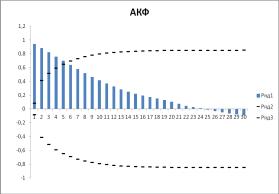
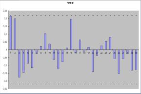
Fig. 1 – ACF and PACF.F for the initial sample.

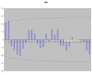
Fig. 2 – ACF and PACF. for a number of first differences.

The calculations of the parameters of the model ARIMA (1,1,0) were conducted by the method of least squares using MS Excel add-in Solver.

The model ARIMA (1,1,0) is

.

The model ARIMA(0,1,2) is

,

where model’s error for level t-1, i.e. the difference between real and model values.

Autoregression model and integrated fluid medium ARIMA (1,1,2) combines the properties of the above two models and has the form

Dispersions of the three discussed models are equal to ARIMA (1,1,0) – 4,894855; ARIMA (0,1,2) – 4,110223; ARIMA (1,1,2) – 3,968714. The model with the lowest variance – ARIMA (1,1,2) is chosen for the prediction.

Point and interval forecast of exchange rate for the model ARIMA (1,1,2) has been compared to the real data (tabl.1). Error forecast was 2.3%, which is quite acceptable.

Table 1 – Comparison with the real value of the course

Period of forecast	Point forecast	The interval of the forecast with theoretical frequency of 95 %		Real value of exchange rate
27.05.2014	11.57711	11.00552	12.1487	11.4673
28.05.2014	11.64003	11.06843	12.21162	11.4635
29.05.2014	11.70691	11.13532	12.2785	11.4648
30.05.2014	11.77379	11.2022	12.34539	11.4271
31.05.2014	11.84068	11.26909	12.41227	11.3999

As a result of work autoregressive models were constructed and implemented short-term forecast error of 2.3%, based on an initial sample of the dynamics of the exchange rate of US dollar against the Ukrainian hryvnia for a fixed period of time.

Reference

1. ARIMA Models and the Box–Jenkins Methodology. Asteriou, Dimitros; Hall, Stephen G/ Applied Econometrics, 2011. Palgrave MacMillan. pp. 265–286.

2. Time series techniques for economists. Terence C. Mills/ Cambridge University Press in Cambridge, New York. 1990, 377p.

3. Spectral analysis for physical applications multitaper and conventional univariate techniques. Donald B. Percival and Andrew T. Walden/ Cambridge University Press in Cambridge, New York, NY, USA, 1993, 583 p.

4. Time series analysis: forecasting and control. Box, G.E.P., and G. M. Jenkins/ Holden Day, San Francisco, CA, 1970, 652 p.

5. Brockwell, P.J., and Davis, R. A. Introduction to time series and forecasting/ Springer,1996, 452 p.

6. Литинский Д.С. Статистическое прогнозирование для построения эффективных торговых стратегий на валютном рынке. Автореф. дисс. канд. экон. наук. Москва, 2003. – 23 с.