P.h.D. Kryuchin O.V.

Tambov State University named after G.R. Derzhavin

The analytic model of the artificial neural networks training using the parallel gradient method

In this paper we will analyze formulas which are used by gradient algorithms (for example the method of the steepest descent, RPROP or QuickProp). We can see that the -th weight at the -th iteration can be calculated by formula

,	(1)

where is the function for calculating weight value , is the step value (for the i-th weight at the I-th iteration) and is the gradient (for its calculation by formulas

	(2)
	(3)

we need vector only) [1, 2]. It means that if weights at the -th iteration is known that it is possibly to calculate values at the -th iteration and it is not necessary to know other weight.

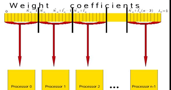
Fig. 1. The scheme of the weights location in IR-elements.

This means that we can divide the weights to number of information resources elements (IR-elements). Such elements can be processes or node of a computer cluster for example. This scheme is shown in picture 1.

If we analyse the information process for the lead and non-lead IR-elements then we can see that the training algorithm consist of few steps [1-3]:

1. forming the ANN structure (with the weights initialization);

2. sending the ANN structure to all non-lead IR-elements;

3. calculating weights vector ;

4. receiving values from all IR-elements;

5. creating vector and calculating inaccuracy value ;

6. checking the stop necessity;

7. sending the stop (or not stop) command to all non-lead IR-elements;

8. if the training has not stop then the sending weights to all IR-elements and go to the third step.

It was the algorithm for the lead IR-element, non-lead use other:

1. receiving the ANN structure from the lead IR-element;

2. calculating weights ;

3. sending weights to the lead IR-element;

4. receiving the stop command;

5. if the training has not end then the receiving full weights vector and go to the second step [4].

If we will analyze formulas which are used by gradient methods then we can see that the the steepest descent and QuickProp execute 3 multiplicative and 2 additive operations and RPROP method executes three multiplicative and one additive operation [1-2, 4]. We should remember that it is necessary () multiplicative and () additive operations for one gradient element calculation. Thus we can count multiplicative and additive operations for one gradient methods iteration (tab. 1).

Table 1. Number of operations for one iteration.

Method	Mult operations number	Add operations number
The steepest descent
QuickProp
RPROP

Each parallel iteration of the information process which uses gradient methods consist of few steps:

· sending weights by the lead IR-element;

· calculating part of gradient and weights;

· sending new weights to the lead IR-element [1].

The first step needs multiplicative and additive operations at the lead IR-element (we will symbol it as ) and at the non-lead (we will symbol it as ). This value consists of operations for the data sending and for the waiting. Operations number which are necessary for the second step are shown in table 2. At the third step the non-lead IR-element executes multiplication and additive operations. The lead IR-element executes multiplicative operations ( for the sending and for the waiting) and additive operations.

Table 2. Number of operations which are executed at the second iteration of information process.

Method	Operations number
	Lead IR-element		Non-lead IR-element
	multiplicative	additive	multiplicative	additive
The st. descent
QuickProp
RPROP

For reduction of addition operations to multiplication operations the coefficient is used. This coefficient value is directly proportional to the time spent for one addition operation and inversely related to the time spent for one multiplication operation. So one multiplication operation needs the time which is necessary for addition operations and one addition operation can be changed to multiplication operations [4].

The first step needs operations at the lead IR-element and operations at other. Values of the second step ( and ) is show in table 2. The third step executes operations at the non-lead IR-element that is why it needs to wait operations before receiving.

So the parallel training information process executes

	(4)

operations. Here information process executes operations of the parallel algorithms ( operations are executed at the last step and is other operations). The efficiency of parallel information process can be calculated by formula

So the analitic model can be wrriten as

for the steepest descent and for QuickProp formula	(6)
	(7)

for the RPROP formula. Here is the iterations number, is the other operations number.

Bibliography

1. Крючин О.В. Разработка параллельных градиентных алгоритмов обучения искусственной нейронной сети // Электронный журнал "Исследовано в России", 096, стр. 1208-1221, 2009 г. // Режим доступа: http://zhurnal.ape.relarn.ru/articles/2009/096.pdf Загл. с экрана.

2. Крючин, О.В. Разработка параллельных эвристических алгоритмов подбора весовых коэффициентов искусственной нейронной сети / О.В. Крючин // Информатика и ее применение. — 2010. — Т. 4, Вып. 2. — C. 53-56.

3. Крючин, О.В. Параллельные алгоритмы обучения искусственных нейронных сетей с использованием градиентных методов / О.В. Крючин // Актуальные вопросы современной науки, техники и технологий: матер. II Всерос. науч.-практ. (заоч.) конф. — М: 2010. — C. 81-86.

4. Крючин, О.В. Параллельные алгоритмы обучения искусственных нейронных сетей / О.В. Крючин // Информационные технологии и математическое моделирование (ИТММ-2009) : матер. VIII Всерос. науч.-практ. конф. с междунар. участием, 12-13 ноября 2009 года. — Томск:, 2009. — Ч. 2. — С. 241-244.