Технические науки/ 4. Транспорт

Assoc. Prof., Ph. D., A. Cherepakha, Assoc. Prof., Ph. D., D. Kopytkov

Kharkov National Automobile and Highway University

The model development to create the virtual cargo delivery routes in the service region

The process to create the routes for delivery of consumer goods is carried out by a transport service enterprise during its operation under conditions of stochastic transport market macro system.

In the model of the route formation it is supposed to allocate the parameters of transport services demand as input parameters, the random effects of the environment are offered to be taken into account by simulation of the random variables of the delivery process technical and operational parameters [1, 2], but the result of the process are suggested to evaluate on the service quality indicators (Figure 1).

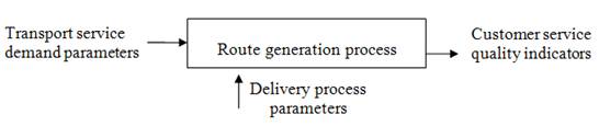
Figure 1 – Cybernetic model to create the delivery routes of consumer goods

The cargo owners are the demand generating subjects of the consumer goods market. Transport service customer when applying a request specifies the source and destination of the goods, in this case, any of the cargo owners can act both as a shipper and as a consignee. A number of shippers S_FO can be defined as a set of the following objects

, (1)

where FO₁, FO₂, …, FO_NFO – cargo owners functioning in the transport market of consumer goods in the region;

N_FO – number of cargo owners in the transport market.

The single cargo owner in the transport market model should be characterized by the location parameters [3] and by the request flow to describe its demand [4]

, (2)

where L_FO – cargo owner location characteristics;

D_FO – request flow characteristics to describe the cargo delivery demand.

Characteristics of the cargo owners geographical location is determined by the coordinates with taking into account the scale [3]. However, if there are some assumptions about the size of the grid for the service region, characteristic of the geographic location can be estimated by the number of the square [3]. For example, in paper [6] in order to describe the geographical location the Location class has been proposed to use. The Location class contains the x and y fields giving the coordinates of the subject on a square grid, the size of which is specified in the areaSize entry.

Associating with the real geographical areas is done in the class with the help of the city and region string fields, containing the name of the locality and the name of the region, respectively. By default, the name of the region is defined as the number of the cell in the grid. To access the value of this entry the Area property is used that is of only the accessory reader and is determined via x, y and the areaSize. Thus, in accordance with the approach [4] to describe the cargo owner geographical location is sufficient to specify the following set of parameters

, (3)

where x, y – cargo owner grid coordinates in the Cartesian system;

N_р – geographic specification level.

The article [3] states that the most important parameter of the transport market model is the geographic specification level N_р. At the same time the geographic specification level refers to the size of a square grid that defines the cargo owner coordinates (the areaSize field in the Location class). The coordinates are determined in accordance with the principle illustrated in Figure 2 (option for N_р = 4). The cargo owner location is

Figure 1 – Service region zoning based on the geographic specification level

This approach to the cargo owner geographical location is sufficient to describe a pair of parameters

, (4)

where k – number of geographical segment of the territory, on which the cargo owner is located.

It should be noted that the approach (4) is only justified in the case of a square grid.

These approaches to the characterization of the geographical segments are interchangeable. Thus, geographical segment number can be determined from a set of parameters (3) as follows

. (5)

Conversely, the x and y coordinates are determined from the set of parameters (4) in the formulas

, (6)

, (7)

where – integer part of a.

Since (3) and (4) are interchangeable, then, resulting from the principle of minimizing the number of parameters of interest, the preferred approach is to determine the characteristics of the cargo owners' geographical location from a pair of the set of parameters .

In general, for a time horizon the demand for cargo transport services is a set of requests

, (8)

where r₁, r₂, …, r_NR – cargo owner requests for transport services;

N_R – number of requests submitted during the period under consideration.

The single request flow describing the demand for delivery of consumer goods [5] should be found from the set of random variables, which are the parameters of single transportation requests. At the same time as the main parameters of the cargo lot, the delivery distance and the request interval were considered [4, 5]. The study [6] was done to outline a zero mileage as a request flow characteristic.

If there are a number of the cargo owners S_FO, thus, there are the geographic location characteristics of each cargo owner, provided that the transport network misalignment ratio close to 1, the delivery distance can be determined from the consignor and consignee geographical location parameters. So, in presence of L_FO it is inappropriate to consider the distance delivery as the request flow parameter. As a necessary characteristic of the delivery request is an indication of the consignor FO_S and consignee FO_O, where , and , the distance of delivery can be estimated as follows

, (9)

,

where x_S, y_S и x_O, y_O – consignor's and consignee's coordinates, respectively.

Obviously, the larger the value N_р and the closer the value of the transport network misalignment factor to 1 (this assumption is usually true in large cities), the formula (9) is more accurate.

The specifics of the consumer goods transportation is expressed in respect of cargo owners’ needs to fulfill the delivery time. Therefore, one of the main characteristics of the consumer goods delivery request is the shipment time expected by the consignee. If it is possible to estimate the request processing duration, then as the request characteristics an allowable service waiting time can be taken, wherein

, (10)

where – consignee-expected shipment time, hours;

– actual duration of the transport service request, hours.

Thus, the consumer goods transportation request is minimally described by a set of the following parameters

, (11)

where – request reception time, hours;

– cargo amount specified in the request, tons.

Except the above-stated parameters, the delivery requests have other characteristics. However, within the routing task the set (11) is sufficient.

Transport service demand D_FF should be determined as a summation of cargo owners' needs

. (12)

In the mathematical model to form the consumer goods delivery routes the transport service demand is the incoming parameter and is described by a set of characteristics

, (13)

where , , and – random variables of the cargo amount, request reception interval, critical waiting time for the request service and delivery distance for the incoming flow of requests.

As criterions to take into account the impact of the environment on the delivery routes formation process, in the model it is proposed to consider the main technical and operational parameters as random variables – the 1 ton loading and unloading time , and the average road speed on the network.

The process of forming the delivery route is considered as the aggregation of the incoming requests to the current point in the group so as to meet the cargo owners’ requirements from one side, and to provide the most effective option service of the incoming request flow – from the other side.

In this context, the delivery route ρ can be mathematically defined as the set of requests, the satisfaction of which is provided by one vehicle during a carrying cycle

, (14)

where r₍₁₎, r₍₁₎, …, r_(Nρ) – cargo owners’ requests to be serviced in the route delivery process;

N_ρ – number of the requests served by one vehicle per ride.

The processing quality of the delivery request flow is determined by trouble-free operation of the hauler and can be estimated as the "number of the requests served-to-the total number of the requests received" ratio

, (15)

where R – cargo owners service level;

n_serv. – number of the requests serviced;

n_Σ – total number of the requests in the flow.

For the set of the routes obtained the number of the requests serviced can be calculated as the sum of capacities of all the sets ρ

, (16)

where – set capacity (number of elements);

N_r – number of the delivery routes obtained.

Accordingly, the total number of the requests in the flow can be found as the sum of the set capacities D_FO that designates the cargo owners’ demand for the time range

. (17)

Thus, the task to obtain the delivery routes for the consumer goods can be formulated as a determination, in the course of client servicing, of such set of the routes S_ρ, for which the value of cargo owners’ service level is optimal

. (18)

The following restrictions must be taken into account when solving the above-stated problem: a) request service time limitation: for the requests aggregated into the route the time interval of their income should not exceed the allowable waiting time for the request received earlier; b) delivery route efficiency limitation: exceeding the dynamic load factor for a set of requests aggregated into the route over the minimum acceptable dynamic load factor (this value is determined by the ratio of market price to the transport service cost); c) cargo amount limitation: there are vehicles used for the delivery, which are of a carrying capacity value that is not less than the maximum possible value of the cargo lot; if the cargo amount exceeds the carrying capacity, such lot is considered as two or more lots with an cargo amount not exceeding the vehicle carrying capacity.

In solving the problem (18) it is proposed to use the following assumptions to the correctness of the mathematical statement: the transport network density for a large city is so high that the misalignment factor is close to 1; a set of shippers is final and cannot be changed during the simulation period: the situation of new customers in the region as well as their disappearance (company dissolution) is not considered; the model presented assumes that the vehicles are of the same body type (vans) used to carry the consumer goods; if the vehicles of different types of body are required when generating the routes it is necessary to consider the flow of requests for the appropriate nature of goods.

REFERENCES

1. Кельтон В. Имитационное моделирование: Пер. с англ. / В. Кельтон, А. Лоу. – СПб. : Питер, 2004. – 847 с.

2. Наумов В. С. Развитие научно-технологических основ экспедиторского обслуживания на автомобильном транспорте: дис. … доктора техн. наук: 05.22.01 / Наумов Виталий Сергеевич. – Харьков, 2013. – 352 с.

3. Наумов В. С. Повышение эффективности информационных систем управления процессами транспортно-экспедиторского обслуживания / В. С. Наумов, О. А. Скорик, А. А. Васютина // Вісник Севастопольського нац. техн. ун-ту: Зб. наук. пр. –2013. – Вип. 143. – С. 211 – 214.

4. Нефедов Н. А. Относительная эффективность развозочных маршрутов / Н. А. Нефедов // Автомоб. трансп.: Сб. науч. тр. – 2002. – Вып. 10 – С. 82 – 84.

5. Naumov V. An approach to modeling of demand on freight forwarding services / V. Naumov, Ie. Nagornyi // Trip Modelling and Demand Forecasting. – Kraków, 2014. – Vol. 1(103). – P. 267 – 277.

6. Наумов В. С. Развитие научно-технологических основ экспедиторского обслуживания на автомобильном транспорте: дис. … доктора техн. наук: 05.22.01 / Наумов Виталий Сергеевич. – Харьков, 2013. – 352 с.