HOVHANNISYAN
T.N.
ON STABILITY OF
SINGLE-INPUT SINGLE-OUTPUT L1 ADAPTIVE CONTROL SYSTEMS
Some issues
concerning the stability of SISO (i.e. having the one input and output)
adaptive control systems for rejecting of external disturbances are discussed.
Based on the properties of positive real transfer functions, it is shown that such
systems are stable for arbitrary large values of the adaptation gain, even in
the case of systems with right half plane zeros.
Keywords: single input single output (SISO) control system, adaptive control,
reference model, stability, positive real system.
The paper examines application of ![]() adaptive control to SISO
control systems [2].
adaptive control to SISO
control systems [2]. ![]() adaptive control was
developed to address some of the deficiencies apparent in Model Reference Adaptive Control (MRAC), as loss of robustness in the presence of fast
adaptation [3, 4].
adaptive control was
developed to address some of the deficiencies apparent in Model Reference Adaptive Control (MRAC), as loss of robustness in the presence of fast
adaptation [3, 4].
As a basic model
of linear one-dimensional systems with constant parameters let consider the system that can be expressed in
the following standard state-space form:
 (1)
(1)
where ![]() is an
is an ![]() -dimensional state vector;
-dimensional state vector; ![]() and
and ![]() are input and output
scalar variables;
are input and output
scalar variables; ![]() is an
is an ![]() constant
matrix,
constant
matrix, ![]() and
and ![]() respectively are
respectively are ![]() -dimensional constant
row- and column-vectors. In what follows, we will assume that system completely
controllable and observable, strictly stable, and, maybe, with Right Half Plane (RHP) transmission zeros.
-dimensional constant
row- and column-vectors. In what follows, we will assume that system completely
controllable and observable, strictly stable, and, maybe, with Right Half Plane (RHP) transmission zeros.
The SISO system (1)
can also be described in the operator form by the ![]() scalar strictly proper rational functions in complex variable
scalar strictly proper rational functions in complex variable ![]() .
.
Generally, the transfer function ![]() is connected with the function
is connected with the function![]() , vectors
, vectors ![]() in (1) by the formula
[5]
in (1) by the formula
[5]
![]() (2)
(2)
where ![]() is an identity function.
is an identity function.
In this article,
we will adhere to the ![]() architecture with state predictor and low-pass filter presented
in [2]. Let an one-dimensional strictly
stable SISO system be described in
state-space by the following equations:
architecture with state predictor and low-pass filter presented
in [2]. Let an one-dimensional strictly
stable SISO system be described in
state-space by the following equations:
 (3)
(3)
where ![]() is a time-dependent scalar
function of unknown external bounded (
is a time-dependent scalar
function of unknown external bounded (![]() ) disturbances that should be rejected by adaptive control,
and all other variables and vectors have the dimensions as in (1).
) disturbances that should be rejected by adaptive control,
and all other variables and vectors have the dimensions as in (1).
The state
predictor has the same structure as the system in (3):
 (4)
(4)
and the only
difference is that the unknown disturbance vector ![]() is replaced by its
estimate
is replaced by its
estimate ![]() .
.
The disturbance
rejection process is governed by the following adaptation law [1]
![]() , (5)
, (5)
where ![]() is the prediction
error,
is the prediction
error, ![]() (
(![]() ) is the solution of the Lyapunov equation
) is the solution of the Lyapunov equation
![]() (6)
(6)
for an arbitrary
symmetric positive definite function ![]() (
(![]() ), and the positive scalar
), and the positive scalar ![]() is called the adaptation gain [1].
is called the adaptation gain [1].
The control signal
![]() of the
system is given in operator form as
of the
system is given in operator form as
![]() , (7)
, (7)
where ![]() is an one-dimensional reference signal,
is an one-dimensional reference signal, ![]() is an static gain,
and
is an static gain,
and ![]() is the transfer function
of a low-pass filter. In the simplest case, the function
is the transfer function
of a low-pass filter. In the simplest case, the function ![]() satisfying the DC
gain condition
satisfying the DC
gain condition ![]() = 1. Its state-space
realization assumes zero initialization.
= 1. Its state-space
realization assumes zero initialization.
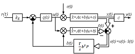
The block diagram
of the control system with the state predictor (4), the adaptive disturbance
rejection law (5), and control signal ![]() (7), is shown in
Figure 1.
(7), is shown in
Figure 1.

Fig
1. Block diagram of the adaptive SISO
control system with the state
predictor and the adaptive disturbance rejection law (5).
Thus, the architecture of the discussed
adaptive control system represents a linear SISO system with integral feedback
and therefore can be investigated by the methods and approaches of linear one variable
feedback control [5, 6]. It should be noted that due to the adopted ![]() scheme with the state
predictor, the transfer function
scheme with the state
predictor, the transfer function ![]() in the control signal
in the control signal
![]() (7) is not present in
the disturbance rejection law (5). Let us consider in more detail the structure
and performance characteristics of the adaptive system in Figure 1. Toward that
end, we introduce the following transfer function
(7) is not present in
the disturbance rejection law (5). Let us consider in more detail the structure
and performance characteristics of the adaptive system in Figure 1. Toward that
end, we introduce the following transfer function
![]() (8)
(8)
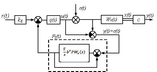
relating the input to the system (1) with the state vector ![]() , and the corresponding (the same) function
, and the corresponding (the same) function ![]() for the state
predictor. Then, the block diagram in Figure 1 can be recast to an equivalent
form in Figure 2.
for the state
predictor. Then, the block diagram in Figure 1 can be recast to an equivalent
form in Figure 2.

Fig
2.
Equivalent block diagram of the adaptive system in Fig 1.
Based on the block diagram in Figure 2 and
equations (2) by considering that ![]() , it is easy to derive the following function equations of
the adaptive system with the state predictor:
, it is easy to derive the following function equations of
the adaptive system with the state predictor:
 , (9)
, (9)
where
 ;
; ![]() . (10)
. (10)
As can be seen
from (10), the output signal of the system ![]() consists of two
components generated, respectively, by the input reference signal
consists of two
components generated, respectively, by the input reference signal ![]() and by the
disturbance
and by the
disturbance ![]() . Since the adaptive SISO system in Figures 1 and 2 is
linear, the superposition principle holds and,
according to the equation (9), the dynamics of the system can be represented by
equivalent block diagram in Figures 3.
. Since the adaptive SISO system in Figures 1 and 2 is
linear, the superposition principle holds and,
according to the equation (9), the dynamics of the system can be represented by
equivalent block diagram in Figures 3.
Let us proceed to
the stability analysis of the adaptive system in Figure 1.

Fig3. Equivalent block diagram of the adaptive system
with
respect to the disturbance ![]() .
.
The block diagram
in Figure 3 contains a negative feedback loop with the open-loop transfer
function ![]() (10) and the following
closed-loop transfer function:
(10) and the following
closed-loop transfer function:
 . (11)
The
characteristic equation of that system is
 , (12)
and, clearly, the
poles of the adaptive system depend on the adaptation gain ![]() , which can be considered as the gain of the open-loop
transfer function
, which can be considered as the gain of the open-loop
transfer function ![]() (10).
(10).
Note now that,
allowing for (8), the system with the transfer function ![]() in (10) can be
written in state-space form as
in (10) can be
written in state-space form as
 (13)
(13)
where
![]() . (14)
. (14)
Taking into
account the form of the function ![]() (13) and recalling
the Kalman-Yakubovich lemma [2-4], we come to a conclusion that
(13) and recalling
the Kalman-Yakubovich lemma [2-4], we come to a conclusion that ![]() belongs to the
so-called Positive Real (PR) transfer
functions and is positive semi-definite (for brevity we shall write
belongs to the
so-called Positive Real (PR) transfer
functions and is positive semi-definite (for brevity we shall write ![]() ) for all real
) for all real ![]() , for which
, for which ![]() is not a pole of any
element of
is not a pole of any
element of ![]() .
.
Example. Consider
a one-dimensional SISO system whit integrating chain and with the transfer function
 (15)
(15)
for which the
transfer function of equivalent adaptive system will be:
 (16)
(16)
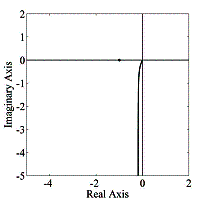
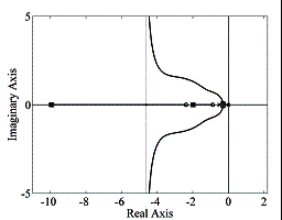
The Nyquist
plots, as well as the root loci of the of the above
function ![]() (16) are shown in
Figure 4.
(16) are shown in
Figure 4.


(a) (b)
Fig
4. Nyquist plots (a) and root loci (b) of ![]() .
.
As can be seen from the graphs in Figure 4, the one-dimensional adaptive
system with the transfer function ![]() is stable for any value
of the adaptation gain
is stable for any value
of the adaptation gain ![]() .
.
References
1. T.
Hovanissyan, N. Vardanyan, E. Kharisov, O. Gasparyan et al. On Application of ![]() Adaptive Control to
Multivariable Control Systems. Part I. General-Type Multivariable Systems // Известия
НАН
и
НПУА. Сер. ТН. – 2014. – Т.67, №4. – С. 434-445.
Adaptive Control to
Multivariable Control Systems. Part I. General-Type Multivariable Systems // Известия
НАН
и
НПУА. Сер. ТН. – 2014. – Т.67, №4. – С. 434-445.
2. Hovakimyan N. and Cao. C. ![]() Adaptive Control
Theory - Guaranteed Robustness with Fast Adaptation. - SIAM, Philadelfia, 2010.
– 340 p.
Adaptive Control
Theory - Guaranteed Robustness with Fast Adaptation. - SIAM, Philadelfia, 2010.
– 340 p.
3. Astrom K.
and Wittenmark B. Adaptive Control. - Addison-Wesley Longman Publishing
Co., Inc., Boston, MA, 1994. -575 p.
4. Ioannou P. and Sun J. Robust Adaptive Control. - Prentice Hall, 1996.
–834p.
5. Skogestad S. and Postlethwaite I. Multivariable
Feedback Control. Analysis and Design. -John Wiley and Sons Ltd., Chichester,
Sussex, UK, 2005. - 595 p.
6. Gasparyan O.
N. Linear and Nonlinear Multivariable Feedback Control: A Classical
Approach. - John Wiley & Sons, UK, 2008. - 354 p.