Student Nechay V

Student Nechay V., Ph.D. Kovalenko M.

National Technical University of Ukraine «Kyiv Polytechnic Institute», Ukraine

The theoretical basis for the development of the field of mathematical models of electrical machines

Lumped parameters are matrices describing electromagnetic properties such as resistance, capacitance, and inductance. In the time-harmonic case the lumped
parameter matrix is either an impedance matrix or an admittance matrix depending on how the model is excited (current or voltage). In a static calculation only the resistive, capacitive, or inductive part of the lumped parameter matrix is obtained.[1] To calculate the lumped parameters, there must be at least two electrodes in the system, one of which must be grounded. Either a voltage or a current can be forced on the electrodes. After the simulation, extract the other property or the energy and use it when calculating the lumped parameter.
There are several available techniques to extract the lumped parameters. Which one to use depends on the physics interface, the parameter of interest, and how the model is solved. The overview of the techniques in this section use a 4-by-4 matrix example for the lumped parameter matrix. This represents a system of at least five electrodes, where four are used as terminals and the rest are grounded, as illustrated in Figur 3-2.[1]

251658240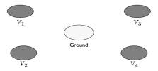 $C:\Users\admin\Desktop\стаття2.png$

Figure 3-2: A five-electrode system with 4 terminals and one ground electrode.

If a system specifies that all electrodes are terminals, the results are redundant matrix elements. This is better understood by considering a two-electrode system. If both electrodes are declared as terminals, a 2-by-2 matrix is obtained for the system. This is clearly too many elements because there is only one unique lumped parameter between the terminals[2]

Forced voltage
If voltages are applied to the terminals, the extracted currents represent elements in the admittance matrix, Y. This matrix determines the relation between the applied voltages and the corresponding currents with the formula[3]

251658240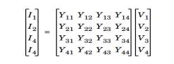 $C:\Users\admin\Desktop\стаття22.png$

so when is nonzero and all other voltages are zero, the vector I is proportional to
the first column of Y.
In electrostatics the current is replaced with charge and the admittance matrix is
replaced with the capacitance matrix

251658240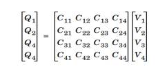 $C:\Users\admin\Desktop\стаття23.png$

Fixed current

It might be necessary to calculate the Z-matrix in a more direct way. Similar to the Y calculation, the Z calculation can be done by forcing the current through one terminal at the time to a nonzero value while the others are set to zero. Then, the columns of the impedance matrix are proportional to the voltage values on all terminals[4]:

251658240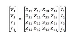 $C:\Users\admin\Desktop\стаття24.png$

In magnetostatics this option means that the energy method is used; see Calculating Lumped Parameters Using the Energy Method below.

Fixed charge

The Electrostatics interface can use total charge instead of total current. This gives the inverted capacitance matrix in a similar manner as the Z and Y matrices.

251658240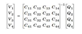 $C:\Users\admin\Desktop\стаття25.png$

Studing Lumped Parameters

To study lumped parameters, use the terminal boundary condition for each electrode.
This boundary condition is available in the following interfaces and the methods
described in the previous section are used to calculate the lumped parameters[4]:
          • Electrostatics. Uses a stationary study and the energy method.
          • Electric Currents. Uses a stationary or frequency domain study type using the method based on Ohm’s law.
          • Magnetic and Electric Fields. For the stationary study the energy method is used. For the frequency domain study type, the method based on Ohm’s law is used.

References:

1. Jianming Jin, The Finite Element Method in Electromagnetics, 2nd ed.,
Wiley-IEEE Press, May 2002.
2. O. Wilson, Introduction to Theory and Design of Sonar Transducers, Peninsula Publishing, 1988.
3. R.K. Wangsness, Electromagnetic Fields, 2nd ed., John Wiley & Sons, 1986.
4. D.K. Cheng, Field and Wave Electromagnetics, 2nd ed., Addison-Wesley, 1991.