Пиль Э.А.

Академик РАЕ, д.т.н., профессор.

DETERMINATION OF CORRELATION DEPENDENCE OF ELLIPSOID SURFACE ON ITS VOLUME

It is well known from the literature on mathematics that during calculation of sphere volume or its surface area it is sufficient to know only one of the values, due to that another may be easily calculated. The issue of identification of correlation dependencies between ellipsoid surface Se and its volume Ve, that is Se = f(Ve) is discussed further in the article. These formulae make it possible to quickly calculate ellipsoidal economic shell surface area which may be interpreted as GDP of a country. The plotted 2D graphs help to visualize the influence of the three variables onto the GDP. The variables remain constant, they decrease and increase.

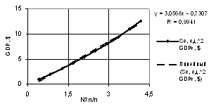
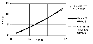
Figures 1 and 2 show two dependencies of GDP with Х1 = 1, Х2 = Х3 = 0.1…1. It is obvious from the presented figures that these dependencies permanently increase up to their maximum value. In this case during calculation of the GDP one may use both linear dependence with the correlation factor of R² = 0.9941, power law dependence with R² = 0.9983.

Fig. 1. GDP = f(X1, X2, X3) Х1 = 1, Х2 = Х3 = 0.1…1	Fig. 2. GDP = f(X1, X2, X3) Х1 = 1, Х2 = Х3 = 0.1…1
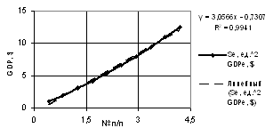
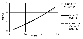
Fig. 3. GDP = f(X1, X2, X3) Х1 = 1, Х2 = Х3 = 1…0.1	Fig. 4. GDP = f(X1, X2, X3) Х1 = 1, Х2 = Х3 = 1…0.1

The next two Figures 3 and 4 display the GDP dependencies when the variables were Х1 = 1, Х2 = Х3 = 1…0.1. Here, the GDP values decrease, and the correlation factors are equal to R² = 0.9941 and R² = 0.9983 accordingly.

Fig. 5. GDP = f(X1, X2, X3) Х1 = 1…10, Х2 = Х3 = 1

Fig. 6. GDP = f(X1, X2, X3) Х1 = 1…10, Х2 = Х3 = 0.1…1

Fig. 7. GDP = f(X1, X2, X3) Х1 = 1…10, Х2 = Х3 = 0.1…1

Fig. 8. GDP = f(X1, X2, X3) Х1 = Х2 = Х3 = 1…10

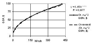
The next Fig. 5 shows that with Х1 = 1…10, Х2 = Х3 = 1 it is expedient to perform the GDP calculation according to the power-law dependence due to the fact that in particular case the correlation factor is substantially huge, and amounts to R² = 0.9977.

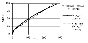
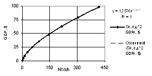
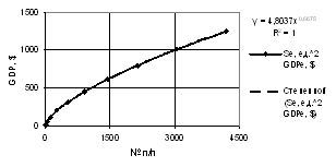
In Figures 6 and 7 the curves of GDP were plotted with Х1 = 1…10, Х2 = Х3 = 0.1…1. It is well seen from the curves that to calculate the GDP one shall use either linear dependence with R² = 0.9745 or the power-law dependence with R² = 1.0.

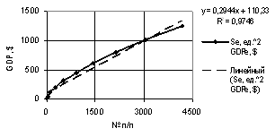
In order to plot the GDP dependencies the following variables' values were used Х1 = Х2 = Х3 = 1…10 in Figures 8 and 9. In order to calculate the GDP value it is necessary to utilize the linear function with R² = 0.9746, or the power-law dependence with R² = 1.0 in these examples.

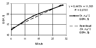
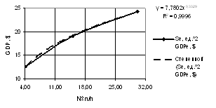
The next two Figures 10 and 11 display the GDP curves plotted with Х1 = 1…3, Х2 = Х3 = 1…0.8. Here, it is quite possible to use linear dependency with R² = 0.9765 during the calculation, or the power-law dependence with R² = 0.9996.

Fig. 9. GDP = f(X1, X2, X3) Х1 = Х2 = Х3 = 1…10

Fig. 10. GDP = f(X1, X2, X3) Х1 = 1…3, Х2 = Х3 = 1…0.8

Fig. 11. GDP = f(X1, X2, X3) Х1 = 1…3, Х2 = Х3 = 1…0.8

Fig. 12. GDP = f(X1, X2, X3) Х1 = 1…6, Х2 = Х3 = 1…0.5

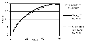
The curve of GDP with Х1 = 1…6, Х2 = Х3 = 1…0.5 was plotted in Figure 12. In this particular case, during the GDP calculation it is necessary to use the power-law dependence with R² = 0.9898.

Fig. 13. GDP = f(X1, X2, X3) Х1 = 7…10, Х2 = Х3 = 0,4…0.1

Fig. 14. GDP = f(X1, X2, X3) Х1 = 1…0.1, Х2 = Х3 = 1

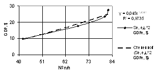
Figure 13 displays the GDP curve plotted with Х1 = 7…10, Х2 = Х3 = 0.4…0.1. Here, it is quite possible to utilize the power-law dependence with R² = 0.9735 during the GDP calculation.

Fig. 15. GDP = f(X1, X2, X3) Х1 = 1…0.1, Х2 = Х3 = 1

Fig. 16. GDP1 GDP = f(X1, X2, X3) Х1 = 1…0.7, Х2 = Х3 = 0.1…0.4

Fig. 17. GDP = f(X1, X2, X3) Х1 = 1…0.7, Х2 = Х3 = 0.1…0.4

Fig. 18. GDP = f(X1, X2, X3) Х1 = 0.6…0.1, Х2 = Х3 = 0.5…1

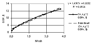
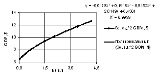
The curves of GDP with Х1 = 1…0.1, Х2 = Х3 = 1 were plotted in Figures 14 and 15. In this example it is necessary to utilize the linear function with R² = 0.9824, or the power-law dependence with R² = 0.9999 during the GDP calculation.

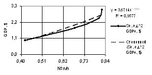
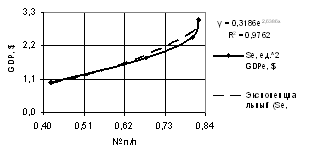
Figures 16 and 17 present the curves plotted with Х1 = 1…0.5, Х2 = Х3 = 0.1…0.6. In this case it is necessary to utilize two functions: the power-law function with R² = 0.9577 or exponential function with R² = 0.9762during the calculation.

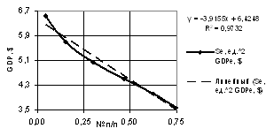
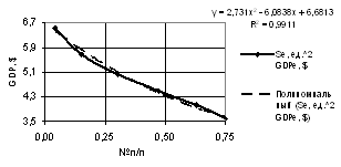
The following two Figures 18 and 19 display the curves plotted with Х1 = 0.6…0.1, Х2 = Х3 = 0.5…1. In this case, it is necessary to utilize the following two functions: the linear function with R² = 0.9732 or polynomial function n = 2 with R² = 0.9911 during the calculation.

Fig. 19. GDP = f(X1, X2, X3) Х1 = 0.6…0.1, Х2 = Х3 = 0.5…1

Fig. 20. GDP = f(X1, X2, X3) Х1 = Х2 = Х3 = 1…0.1

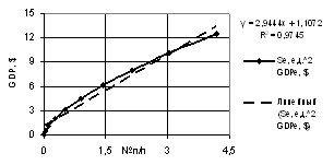
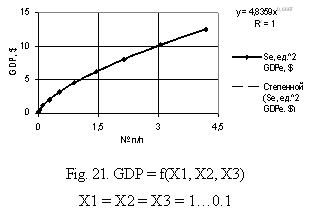
The two Figures 20 and 21 display the GDP curves plotted with the same values of variables Х1 = Х2 = Х3 = 1…0.1. In this case, it is necessary to utilize the following two functions: the linear function with R² = 0.9745 or the power-law function with correlation factor of R² = 1.0 during the GDP calculation.

Basing on the information and presented graphs, the priorities during the GDP calculations are the following: linear and power-law functions take the first place, polynomial and exponential functions follow.