Пиль Э.А.
Академик РАЕ, д.т.н., профессор
THEORY OF THE FINANCIAL CRISES (PART III)
Earlier in his articles the author has shown that in
order to describe the economic processes that occur in the economy of a country
it is possible to apply the shell theory, in its application to the spheres [1,
4]. Besides, the author has also described in the articles the boundaries of
existence of economic shells of small-, medium- and big-sized businesses which
may be influenced by both external and internal forces [2, 3]. The author
suggests in the following article to employ ellipsoidal economic shell, and, to
be more specific - its volume which will make it
possible to use six different variables during calculation of the GDP.
Gross domestic product can be calculated by the three
following methods:
1.
as the sum of gross value added (production method);
2.
as the sum of end-use components (end-use method);
3.
as the sum of primary income (distribution method).
In this case the various variables may be used in the
calculation, in particular such as: consuming capacity, investments,
governmental expenditures, exports, imports and the like. In the material
presented below the calculation formula of volume of the economic shell Veu was
used, to which corresponds the GDP of the country, that is Veu (GDPeu)
= f(Х1, Х2,
Х3, Х4, Х5, Х6). Here Х1, Х2, Х3,
Х4, Х5 and Х6 are the variables which have an impact on the GDP of the country.
By analysing the formula it
is possible to identify the variables' characteristics which influence on the Veu (GDPeu),
and which will be as follows:
·
where the Х1
variable is increased, the economic shell volume Veu GDPeu
increases too;
·
where
the Х2
variable is increased, the economic shell volume Veu (GDPeu)
increases more profoundly compared to the increase of variable X1;
·
where the Х3
variable is increased, the economic shell volume Veu (GDPeu)
decreases;
·
where the Х4
variable is increased, the economic shell volume Veu (GDPeu)
increases. In such a case the X4 variable may approach to numeral one only asymptotically;
·
where the Х5
variable is increased, the economic shell volume Veu (GDPeu)
decreases;
·
where the Х6
variable is increased, the economic shell volume Veu (GDPeu)
increases less profoundly compared to the increase of variable X4. In such a
case the X6 variable may approach to numeral one only asymptotically.
It should immediately be noted that during calculation
and plotting of construction drawings, the parameters Х1,
Х2, Х3, Х4, Х5 and Х6 could be constant values, increase or decrease by 10 times. On the basis
of the calculations made, 82 graphics were built, which can be divided into the
four following groups:
• parameter values Х1, Х2, Х3, Х4, Х5
and Х6
increase and are constant;
• parameter values Х1, Х2, Х3, Х4, Х5
and Х6
decrease and are constant;
• parameter values Х1, Х2, Х3, Х4, Х5
and Х6
decrease and increase;
• parameter values Х1, Х2, Х3, Х4, Х5
and Х6
are constant, they decrease and increase.
It is worth mentioning here in this context that the
number of the graphs that may be plotted with the six variables is
significantly greater. Therefore the author has selected such options of the
variables' values which will more precisely show the variables' influence onto
the GDP calculation.
Figure 1 shows the 2D graph of Veu (GDPeu)
dependency with Х1 = 1, Х2 = Х3 = Х5 = 1…10, Х4 = Х6 = 0.1…0.99 from which it is
clear that the Veu
values initially decrease by 11.42 times, and afterwards increase by 6.77
times. The minimal value of the Veu (GDPeu) falls on point 7, and is equal to 0.16.
Figure 2 shows two 3D-graphs which give the possibility to more illustratively
present the changes in the Veu. In this particular case it is essential to
have the values of the extreme points, since with such values the Veu
value, and finally the GDPeu, will be maximal.
Fig. 1. Dependence Veu (GDPeu) = f(Х1, Х2, Х3,
Х4, Х5, Х6)
when Х1 = 1, Х2 = Х3 = Х5 = 1…10, Х4 = Х6 =
0.1…0.99
|
a |
b |
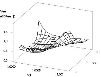
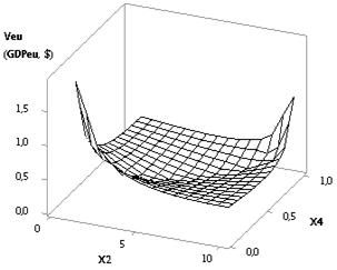
Fig. 2. 3D-graphics: a - Veu (GDPeu) = f(Х1, Х2); b - Veu (GDPeu) = f(Х2, Х4)
when Х1 = 1, Х2 = Х3 = Х5 = 1…10, Х4 = Х6 = 0.1…0.99
Fig. 3. Dependence Veu (GDPeu) = f(Х1, Х2, Х3,
Х4, Х5, Х6)
when Х1 = Х2 = 1…10, Х3 = Х5 = 1, Х4 = Х6 =
0.99
|
a |
b |
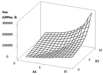
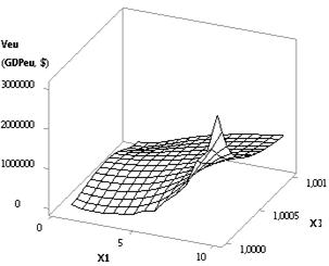
Fig. 4. 3D-graphics: a - Veu (GDPeu) = f(Х1, Х2); b - Veu (GDPeu) = f(Х1, Х3)
when Х1 = Х2 = 1…10, Х3 = Х5 = 1, Х4 = Х6 =
0.99
Fig.
5. Dependence Veu (GDPeu) = f(Х1, Х2, Х3,
Х4, Х5, Х6)
when Х1 = 1, Х2 = Х3 = Х5 = 1…0.1, Х4 = Х6
= 0.99…0.1
From the next Figure 3 it is
clear that when Х1 = Х2 =
1…10, Х3 = Х5 = 1, Х4 = Х6 = 0.99 the plotted curve Veu grows in full
swing from the value 95.27 up to 3.01Е+06, that is - it increases by 31622.78 times. Figure 4 shows
two types of the present dependency in way of 3D-graphs. Such option is the
most preferred one, since the biggest increase of the values Veu (GDPeu)
takes place under the influence of external forces.
In Figure 5 we may see that the Veu curve plotted has also the minimum of 14.08 in
point 4, after which its values increase. This figure was plotted under the
following values of the variables: Х1 = 1, Х2 = Х3 = Х5 = 1…0.1, Х4 = Х6 = 0.99…0.1. Here, it is also important to select the variables in extreme points,
since in this case the economy of the country in question will have the maximal
values of the Veu.
The depicted Veu
curve plotted in Figure 5 is presented by two 3D-graphs in Figure 6.
|
a |
b |
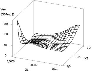
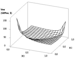
Fig. 6. 3D-graphics: a - Veu (GDPeu) = f(Х1, Х2); b - Veu (GDPeu) = f(Х2, Х3)
when Х1 = 1, Х2 = Х3 = Х5 = 1…0.1, Х4 = Х6
= 0.99…0.1
Fig.
7. Dependence Veu (GDPeu) = f(Х1, Х2, Х3,
Х4, Х5, Х6)
when Х1 = 1…10, Х2 = 1…0.1, Х3 = Х5 = 1, Х4
= Х6 = 0.99
Figure 7 depicts the Veu curve which has
its maximum of 261.41 in point 4. Consequently, use of the following values of
variables Х1 =
1…10, Х2 =
1…0.1, Х3 = Х5 = 1, Х4 = Х6 = 0.99 is quite expedient at the
values which are close to the maximal ones. Figure 8 shows three examples of
3-dimensional surfaces Veu
(GDPeu)
= f(Х1, Х2,
Х3, Х4, Х5, Х6).
As it is clear from Figure 9, here the Veu
values have their minimum of 80.18 in point 2, after which they grow up to
246.73, and then drop down to zero, since the Veu calculations have
no solutions with the subsequent values of the variables. During plotting of
Figures 9 and 10 the following variables were used: Х1 = 1…10, Х2 = Х3 = Х5 = 1…0.1, Х4 = 0.99…0.1, Х6 = 0.99. Here, the four types of
3D-graphs are shown, which are presented in Figure 10.
|
a |
b |
|
c |
|
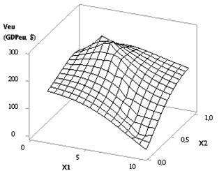
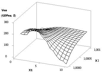
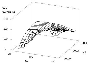
Fig. 8. 3D-graphics: a - Veu (GDPeu) = f(Х1, Х2); b - Veu (GDPeu) = f(Х1, Х3)
c - Veu (GDPeu) = f(Х2, Х3)
when Х1 = 1…10, Х2 = 1…0.1, Х3 = Х5 = 1, Х4
= Х6 = 0.99
Fig.
9. Dependence Veu (GDPeu) = f(Х1, Х2, Х3,
Х4, Х5, Х6)
when Х1 = 1…10, Х2 = Х3 = Х5 = 1…0.1, Х4 = 0.99…0.1, Х6 = 0.99
|
|
|
|
|
d |
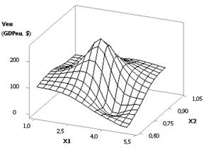
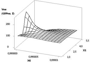
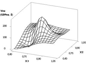
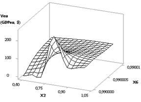
Fig. 10. 3D-graphics: a - Veu (GDPeu)
= f(Х1, Х2); b - Veu (GDPeu)
= f(Х6, Х1);
c - Veu (GDPeu) = f(Х3, Х2); d - Veu (GDPeu) = f(Х2, Х6);
when Х1 = 1…10, Х2 = Х3 = Х5 = 1…0.1, Х4 = 0.99…0.1, Х6 = 0.99
Fig.
11. Dependence Veu (GDPeu) = f(Х1, Х2, Х3,
Х4, Х5, Х6)
when Х1 = 1…0.1, Х2 = 1…10, Х3 = Х5 = 1, Х4 = Х6 = 0.99
From the following Figure 11 it is obvious that the
plotted Veu
- curve has its maximal value of Veu = 8266.58 in point 7. This particular Figure
was plotted with Х1 = 1…0.1, Х2 = 1…10, Х3 = Х5 =
1, Х4 = Х6 = 0.99.
The two Figures 12 show the way how the presented Veu-curve changes in
the three-dimensional space.
|
a |
b |
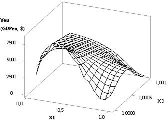
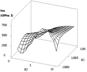
Fig. 12. 3D-graphics: a - Veu (GDPeu) = f(Х1, Х3); b - Veu (GDPeu) = f(Х2, Х3)
when Х1 = 1…0.1, Х2 = 1…10, Х3 = Х5 = 1, Х4 = Х6 = 0.99
Fig.
13. Dependence Veu (GDPeu) = f(Х1, Х2, Х3,
Х4, Х5, Х6)
when Х1 = 1, Х2 = Х5 = 1…0.1, Х3 = 1…10, Х4 = 0.1…0.99, Х6 = 0.99
The following Figure 13
represents the Veu (GDPeu) curve when Х1 = 1, Х2 = Х5 = 1…0.1, Х3 = 1…10, Х4 = 0,1…0.99, Х6 = 0.99. From this 2D-graph it is seen that the
plotted curve has its minimum of 2.7 in point 2, after which is gets its
maximum of 3.34 in point 3, and next their values drop down to zero. The last
Figure 14 displays the four types of three-dimensional surfaces Veu (GDPeu) for
the curve plotted in Figure 13.
After the calculations were completed, their results
were combined into the summary table, which gave totally 109 lines, in spite of
the fact that only 82 two-dimensional graphs have been plotted. This resulted
from the fact that a number of the plotted graphs had their maximums and
minimums. The relationships were introduced into this summary table as the
following:
• Veub…Veuf, where Veub
- is the initial volume value of financial shell, unit3; Veuf - is the final value of the volume of financial shell, unit3;
• Veuf/Veub
- is the relation of financial shell final volume value to its initial
value.
|
a |
b |
|
c |
d |
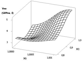
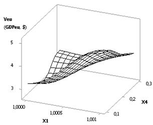
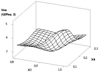
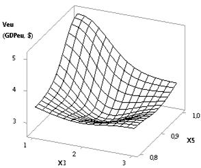
Fig. 14. 3D-graphics: a - Veu (GDPeu)
= f(Х1, Х2); b - Veu (GDPeu)
= f(Х1, Х4);
c - Veu (GDPeu) = f(Х2, Х4); d - Veu (GDPeu) = f(Х3, Х5);
when Х1 = 1, Х2 = 1…0.1, Х3 = 1…10, Х4 = 0.1…0.99, Х5 = 1…0.1,
Х6 = 0.99
The ratio of finite volume of the economic shell Veuf to the initial Veub
shows by how many times the volume of the economic shell increased (decreased),
that is Veu (GDPeu), under the influence
of various external forces onto the one. Hence, by obtaining these data we may
choose such values of variables Х1, Х2, Х3, Х4, Х5 and Х6, with which the volume
of the economic shell remains invariable, or even grows further under influence
of external forces. This means that in case of economical crisis, the selected
values of the variables will make it possible to stay on the previous level, or
even to increase the GDP of the country. After the Table had been plotted with
its 109 lines available, it was converted in the following way, by having left
only those values where Veuf/Veub ≥ 1. On the basis of such conversion
the final table had been obtained, which contained 62 lines, which then was
shortened down to 40 lines where the values of the ratio Veuf/Veub
in column 8 were located in descending order (refer to Table 1). As it is seen
from the calculated data in Table 1 the ratios Veuf/Veub ≥ 1 start with 53 and end up with
1.4. This indicates that for the example in question the economy may maximally
increase even under the pressure onto the ellipsoidal economic shell as by
53376.24 times, as compared to the initial state with the following values of
the variables, being Х1 = Х2 =
1…10, Х3 = Х5 = 1, Х4 = Х6 = 0.99. Yet maximal growth of
the economic shell will take place in this particular case with 1.49 at Х1 = 1, Х2 = Х3 = 1…0.1, Х4 = 0.1…0.99, Х5 = 1…10, Х6 = 0.99.
The next Table 2 was plotted on the basis of Table 1
in which the data obtained were split into groups by the number of variables
used. As it is seen
from Table 2 the data presented in it were grouped into 6 groups, starting from
the group with one variable, and ending up with the group where all the
variables were used. It is also seen from this table that the biggest group was
presented by the group containing four variables.
Due to the fact that variable X2 characterises the thickness of the economic shell it means
that if it was accepted as the single unit (Х2 = 1) then Table 2 will change into Table 3 where
there will be only 15 lines instead of 40. The X2 variable may be characterized as the ratio of national
currency exchange rate to a currency used in international settlements (US
dollar, Euro, etc.).
As a result the following conclusions may be made:
1.
Utilization of different
values of the variables makes it feasible to increase the GDP of the country,
and in a number of instances to increase quite significantly and to lift the
economy out of crisis;
2.
During selection of the
variables' values it is necessary to select such group in which the number of
variables under consideration is minimal;
During selection of the variables' values it is
necessary to select such variables which are less subject to changes.
|
Table 1. Statistics
of theoretical relation Veuf /Veub, where Veuf /Veub
≥ 1 in descending order |
||||||||
|
No.
in sequence |
Х1 |
Х2 |
Х3 |
Х4 |
Х5 |
Х6 |
Veub…Veuf (GDPeub…GDPeuf. $) |
Veuf / Veub (GDPeuf / GDPeub) |
|
1 |
2 |
3 |
4 |
5 |
6 |
7 |
8 |
|
|
1. |
1…10 |
1…10 |
1…0.1 |
0.99…0.1 |
1 |
0.99 |
95.27…5.08E+06 |
53376.24 |
|
2. |
1 |
1…10 |
1…0.1 |
0.99…0.1 |
1…0.1 |
0.99…0.1 |
95.27…5.08E+06 |
53376.24 |
|
3. |
1…10 |
1…10 |
1 |
0.99 |
1 |
0.99 |
95.27…3.01E+06 |
31622.78 |
|
4. |
1 |
1…10 |
1…0.1 |
0.99 |
1 |
0.99 |
95.27…3.01E+06 |
31622.78 |
|
5. |
1 |
1…10 |
1…0.1 |
0.1…0.99 |
1 |
0.99 |
5.08…95266.87 |
18734.93 |
|
6. |
1…10 |
1…10 |
1…10 |
0.1…0.99 |
1 |
0.99 |
5.08…95266.87 |
18734.93 |
|
7. |
1…0.1 |
1…10 |
1…0.1 |
0.1…0.99 |
1 |
0.99 |
5.08…9.5E+04 |
18734.93 |
|
8. |
1 |
1…10 |
1…0.1 |
0.1…0.99 |
1…0.1 |
0.1…0.99 |
1.87…27568.22 |
14778.39 |
|
9. |
1 |
1 |
1…0.1 |
0.99…0.1 |
1…0.1 |
0.99…0.1 |
26.51…1.61E+05 |
6065.80 |
|
10.
|
1…10 |
1 |
1…0.1 |
0.99…0.1 |
1…0.1 |
0.99…0.1 |
64.02…1.61E+05 |
2511.77 |
|
11.
|
1 |
1…10 |
1…10 |
0.1…0.99 |
1 |
0.1…0.99 |
1.87…3012.60 |
1614.95 |
|
12.
|
1 |
1 |
1…10 |
0.1…0.99 |
1…0.1 |
0.99…0.1 |
2.03…3012.60 |
1481.61 |
|
13.
|
1…10 |
1 |
1…0.1 |
0.1…0.99 |
1…0.1 |
0.1…0.99 |
1.87…1875.78 |
1005.54 |
|
14.
|
1 |
1…10 |
1 |
0.99 |
1 |
0.99 |
95.27…95266.87 |
1000.0 |
|
15.
|
1 |
1 |
1 |
0.99 |
1…0.1 |
0.99…0.1 |
95.27…95266.87 |
1000.0 |
|
16.
|
1…10 |
1…10 |
1…10 |
0.99 |
1 |
0.99 |
95.27…95266.87 |
1000.0 |
|
17.
|
1 |
1…10 |
1…0.1 |
0.99…0.1 |
1…0.1 |
0.1…0.99 |
34.95…24559.53 |
702.73 |
|
18.
|
1…10 |
1 |
1…10 |
0.99…0.1 |
1 |
0.99 |
3012.60 |
592.45 |
|
19.
|
1 |
1 |
1 |
0.99…0.1 |
1…0.1 |
0.99…0.1 |
20.67…5084.99 |
246.05 |
|
20.
|
1 |
1…10 |
1…0.1 |
0.1…0.99 |
1…0.1 |
0.99 |
5.08…916.0 |
180.14 |
|
21.
|
1…10 |
1…0.1 |
1…0.1 |
0.99…0.1 |
1…0.1 |
0.99…0.1 |
54.66…5084.99 |
93.03 |
|
22.
|
1…0.1 |
1…10 |
1 |
0.99 |
1 |
0.99 |
95.27…8266.58 |
86.77 |
|
23.
|
1 |
1 |
1 |
0.1…0.99 |
1…0.1 |
0.1…0.99 |
1.87…127.63 |
68.42 |
|
24.
|
1…10 |
1…10 |
1…10 |
0.99…0.1 |
1 |
0.99 |
95.27…5084.99 |
53.38 |
|
25.
|
1 |
1 |
1 |
0.99 |
1…0.1 |
0.1…0.99 |
34.95…1738.10 |
49.73 |
|
26.
|
1 |
1…0.1 |
1…10 |
0.1…0.99 |
1…0.1 |
0.99 |
5.08…176.28 |
34.67 |
|
27.
|
1 |
1 |
1…0.1 |
0.1…0.99 |
1…10 |
0.99…0.1 |
0.034…1.10 |
32.72 |
|
28.
|
1 |
1…10 |
1…10 |
0.99 |
1 |
0.99 |
95.27…3012.60 |
31.62 |
|
29.
|
1…10 |
1…0.1 |
1…0.1 |
0.1…0.99 |
1 |
0.99 |
5.08…95.27 |
18.73 |
|
30.
|
1 |
1 |
1 |
0.99…0.1 |
1…0.1 |
0.1…0.99 |
8.38…113.70 |
13.57 |
|
31.
|
1 |
1…0.1 |
1…0.1 |
0.99…0.1 |
1…0.1 |
0.99…0.1 |
14.08…160.80 |
11.42 |
|
32.
|
1 |
1…10 |
1…0.1 |
0.99…0.1 |
1…10 |
0.99 |
5.37…58.99 |
10.98 |
|
33.
|
1 |
1…10 |
1…10 |
0.1…0.99 |
1…10 |
0.99 |
0.16…1.11 |
6.71 |
|
34.
|
1 |
1 |
1…10 |
0.99…0.1 |
1…0.1 |
0.1…0.99 |
1.42…7.74 |
5.44 |
|
35.
|
1…10 |
1…0.1 |
1…0.1 |
0.99 |
1 |
0.99 |
95.27…495.02 |
5.20 |
|
36.
|
1 |
1 |
1 |
0.1…0.99 |
1…10 |
0.99…0.1 |
0.0075…0.03 |
4.61 |
|
37.
|
1 |
1 |
1…10 |
0.1…0.99 |
1…10 |
0.1…0.99 |
0.00031…0.001 |
3.59 |
|
38.
|
1…10 |
1…0.1 |
1…0.1 |
0.99…0.1 |
1…0.1 |
0.99 |
80.18…246.73 |
3.08 |
|
39.
|
1 |
1 |
1 |
0.99 |
1 |
0.1…0.99 |
34.95…95.27 |
2.73 |
|
40.
|
1 |
1…0.1 |
1…0.1 |
0.1…0.99 |
1…10 |
0.99 |
0.0007…0.0011 |
1.49 |
|
Table 2. The statistics of variable
parameters for Veuf
/Veub,
where Veuf /Veub ≥ 1 in
descending order for groups |
||||||||
|
No. in sequence |
Х1 |
Х2 |
Х3 |
Х4 |
Х5 |
Х6 |
Veub…Veuf (GDPeub…GDPeuf. $) |
Veuf / Veub (GDPeuf / GDPeub) |
|
1 |
2 |
3 |
4 |
5 |
6 |
7 |
8 |
|
|
1
variable |
||||||||
|
1. |
1 |
1…10 |
1 |
0.99 |
1 |
0.99 |
95.27…95266.87 |
1000.0 |
|
2. |
1 |
1 |
1 |
0.99 |
1 |
0.1…0.99 |
34.95…95.27 |
2.73 |
|
2
variables |
||||||||
|
3. |
1…10 |
1…10 |
1 |
0.99 |
1 |
0.99 |
95.27…3.01E+06 |
31622.78 |
|
4. |
1 |
1…10 |
1…0.1 |
0.99 |
1 |
0.99 |
95.27…3.01E+06 |
31622.78 |
|
5. |
1 |
1 |
1 |
0.99 |
1…0.1 |
0.99…0.1 |
95.27…95266.87 |
1000.0 |
|
6. |
1…0.1 |
1…10 |
1 |
0.99 |
1 |
0.99 |
95.27…8266.58 |
86.77 |
|
7. |
1 |
1 |
1 |
0.99 |
1…0.1 |
0.1…0.99 |
34.95…1738.10 |
49.73 |
|
8. |
1 |
1…10 |
1…10 |
0.99 |
1 |
0.99 |
95.27…3012.60 |
31.62 |
|
3
variables |
||||||||
|
9. |
1 |
1…10 |
1…0.1 |
0.1…0.99 |
1 |
0.99 |
5.08…95266.87 |
18734.93 |
|
10.
|
1…10 |
1…10 |
1…10 |
0.99 |
1 |
0.99 |
95.27…95266.87 |
1000.0 |
|
11.
|
1…10 |
1 |
1…10 |
0.99…0.1 |
1 |
0.99 |
3012.60 |
592.45 |
|
12.
|
1 |
1 |
1 |
0.99…0.1 |
1…0.1 |
0.99…0.1 |
20.67…5084.99 |
246.05 |
|
13.
|
1 |
1 |
1 |
0.1…0.99 |
1…0.1 |
0.1…0.99 |
1.87…127.63 |
68.42 |
|
14.
|
1 |
1 |
1 |
0.99…0.1 |
1…0.1 |
0.1…0.99 |
8.38…113.70 |
13.57 |
|
15.
|
1…10 |
1…0.1 |
1…0.1 |
0.99 |
1 |
0.99 |
95.27…495.02 |
5.20 |
|
16.
|
1 |
1 |
1 |
0.1…0.99 |
1…10 |
0.99…0.1 |
0.0075…0.03 |
4.61 |
|
4
variables |
||||||||
|
17.
|
1…10 |
1…10 |
1…0.1 |
0.99…0.1 |
1 |
0.99 |
95.27…5.08E+06 |
53376.24 |
|
18.
|
1…10 |
1…10 |
1…10 |
0.1…0.99 |
1 |
0.99 |
5.08…95266.87 |
18734.93 |
|
19.
|
1…0.1 |
1…10 |
1…0.1 |
0.1…0.99 |
1 |
0.99 |
5.08…9.5E+04 |
18734.93 |
|
20.
|
1 |
1 |
1…0.1 |
0.99…0.1 |
1…0.1 |
0.99…0.1 |
26.51…1.61E+05 |
6065.8 |
|
21.
|
1 |
1…10 |
1…10 |
0.1…0.99 |
1 |
0.1…0.99 |
1.87…3012.60 |
1614.95 |
|
22.
|
1 |
1 |
1…10 |
0.1…0.99 |
1…0.1 |
0.99…0.1 |
2.03…3012.60 |
1481.61 |
|
23.
|
1 |
1…10 |
1…0.1 |
0.1…0.99 |
1…0.1 |
0.99 |
5.08…916.0 |
180.14 |
|
24.
|
1…10 |
1…10 |
1…10 |
0.99…0.1 |
1 |
0.99 |
95.27…5084.99 |
53.38 |
|
25.
|
1 |
1…0.1 |
1…10 |
0.1…0.99 |
1…0.1 |
0.99 |
5.08…176.28 |
34.67 |
|
26.
|
1 |
1 |
1…0.1 |
0.1…0.99 |
1…10 |
0.99…0.1 |
0.034…1.10 |
32.72 |
|
27.
|
1…10 |
1…0.1 |
1…0.1 |
0.1…0.99 |
1 |
0.99 |
5.08…95.27 |
18.73 |
|
28.
|
1 |
1…10 |
1…0.1 |
0.99…0.1 |
1…10 |
0.99 |
5.37…58.99 |
10.98 |
|
29.
|
1 |
1…10 |
1…10 |
0.1…0.99 |
1…10 |
0.99 |
0.16…1.11 |
6.71 |
|
30.
|
1 |
1 |
1…10 |
0.99…0.1 |
1…0.1 |
0.1…0.99 |
1.42…7.74 |
5.44 |
|
31.
|
1 |
1 |
1…10 |
0.1…0.99 |
1…10 |
0.1…0.99 |
0.00031…0.001 |
3.59 |
|
32.
|
1 |
1…0.1 |
1…0.1 |
0.1…0.99 |
1…10 |
0.99 |
0.0007…0.0011 |
1.49 |
|
5
variables |
||||||||
|
33.
|
1 |
1…10 |
1…0.1 |
0.99…0.1 |
1…0.1 |
0.99…0.1 |
95.27…5.08E+06 |
53376.24 |
|
34.
|
1 |
1…10 |
1…0.1 |
0.1…0.99 |
1…0.1 |
0.1…0.99 |
1.87…27568.22 |
14778.39 |
|
35.
|
1…10 |
1 |
1…0.1 |
0.99…0.1 |
1…0.1 |
0.99…0.1 |
64.02…1.61E+05 |
2511.77 |
|
36.
|
1…10 |
1 |
1…0.1 |
0.1…0.99 |
1…0.1 |
0.1…0.99 |
1.87…1875.78 |
1005.54 |
|
37.
|
1 |
1…10 |
1…0.1 |
0.99…0.1 |
1…0.1 |
0.1…0.99 |
34.95…24559.53 |
702.73 |
|
38.
|
1 |
1…0.1 |
1…0.1 |
0.99…0.1 |
1…0.1 |
0.99…0.1 |
14.08…160.80 |
11.42 |
|
39.
|
1…10 |
1…0.1 |
1…0.1 |
0.99…0.1 |
1…0.1 |
0.99 |
80.18…246.73 |
3.08 |
|
all the variables |
||||||||
|
40.
|
1…10 |
1…0.1 |
1…0.1 |
0.99…0.1 |
1…0.1 |
0.99…0.1 |
54.66…5084.99 |
93.03 |
|
Table 3. The statistics of variable
parameters for Veuf /Veub, where
Veuf /Veub ≥ 1 and Х2 = 1 in descending order
for groups |
||||||||
|
No. in sequence |
Х1 |
Х2 |
Х3 |
Х4 |
Х5 |
Х6 |
Veub…Veuf (GDPeub…GDPeuf. $) |
Veuf / Veub (GDPeuf / GDPeub) |
|
1 |
2 |
3 |
4 |
5 |
6 |
7 |
8 |
|
|
1
variable |
||||||||
|
1. |
1 |
1 |
1 |
0.99 |
1 |
0.1…0.99 |
34.95…95.27 |
2.73 |
|
2 variables |
||||||||
|
2. |
1 |
1 |
1 |
0.99 |
1…0.1 |
0.99…0.1 |
95.27…95266.87 |
1000.0 |
|
3. |
1 |
1 |
1 |
0.99 |
1…0.1 |
0.1…0.99 |
34.95…1738.10 |
49.73 |
|
3 variables |
||||||||
|
4. |
1…10 |
1 |
1…10 |
0.99…0.1 |
1 |
0.99 |
3012.60 |
592.45 |
|
5. |
1 |
1 |
1 |
0.99…0.1 |
1…0.1 |
0.99…0.1 |
20.67…5084.99 |
246.05 |
|
6. |
1 |
1 |
1 |
0.1…0.99 |
1…0.1 |
0.1…0.99 |
1.87…127.63 |
68.42 |
|
7. |
1 |
1 |
1 |
0.99…0.1 |
1…0.1 |
0.1…0.99 |
8.38…113.70 |
13.57 |
|
8. |
1 |
1 |
1 |
0.1…0.99 |
1…10 |
0.99…0.1 |
0.0075…0.03 |
4.61 |
|
4 variables |
||||||||
|
9. |
1 |
1 |
1…0.1 |
0.99…0.1 |
1…0.1 |
0.99…0.1 |
26.51…1.61E+05 |
6065.8 |
|
10.
|
1 |
1 |
1…10 |
0.1…0.99 |
1…0.1 |
0.99…0.1 |
2.03…3012.60 |
1481.61 |
|
11.
|
1 |
1 |
1…0.1 |
0.1…0.99 |
1…10 |
0.99…0.1 |
0.034…1.10 |
32.72 |
|
12.
|
1 |
1 |
1…10 |
0.99…0.1 |
1…0.1 |
0.1…0.99 |
1.42…7.74 |
5.44 |
|
13.
|
1 |
1 |
1…10 |
0.1…0.99 |
1…10 |
0.1…0.99 |
0.00031…0.001 |
3.59 |
|
5 variables |
||||||||
|
14.
|
1…10 |
1 |
1…0.1 |
0.99…0.1 |
1…0.1 |
0.99…0.1 |
64.02…1.61E+05 |
2511.77 |
|
15.
|
1…10 |
1 |
1…0.1 |
0.1…0.99 |
1…0.1 |
0.1…0.99 |
1.87…1875.78 |
1005.54 |
REFERENCES
1.
Pil E. A. Use of the shells' theory for purposes of description of
processes taking place in economy // Альманах современной науки и образования (Almanac of modern science and
education). 2009. №3. P. 137-139
2.
Pil E. A. Influence of different variables onto economic shell of the
country // Альманах современной науки и образования (Almanac of modern science and
education). 2012. №12 (67).
P. 123-126
3. Pil
E.A. Variants of macroeconomics development after being affected by different
forces // Materials of the XII International scientific and practical
conference, «Prospect of world science - 2016», 30 July – 7 August. 2016 Volume
2. Economic science. Governance. Sheffield. Science and education. LTD. UK –
100 p. – P. 17–32
4.
Pil E.A. Theory of the financial crises // International Scientific and
Practical Conference. Topical researches of the world science (June 20–21,
2015) Vol. IV Dubai, UAE. – 2015 – Р. 44–56