Pil E.A.

Academic RANH, dr. sc., professor, Saint-Petersburg

GDP CALCULATION WITH ONE VARIABLE HAVING A NEGATIVE VALUE

This article examines an issue of calculation of the gross domestic product under influence of four variables, one of which has a negative value. The calculations served as a basis for plotting 2D and 3D graphs.

The article below shows how the negative values of one parameter out of four influence the GDP, while other parameters have positive values, grow or diminish by a factor of 10 times. In our calculations, the variable X4 has negative values. Thus, at issue is the GDP change V_su (GDP) = f (Х1, Х2, Х3, Х4). Here GDP is understood as the volume of the economic shell V_su. In this case, the values of the variable X4 may be viewed as a key rate or taxes, because their values may not equal 1. In our example, let's assume hypothetically that the variable X4 is a key rate. The State may theoretically adopt negative taxes, though there was no such precedent in practice.

Recently, articles on negative interest rates have appeared online, where such rates are referred to as the 'key rate' [1, 2, 3, 4]. This article treats calculations related to the theory of economic crises.

Figure 1 shows a 2D graph which was plotted with the following values of variables: Х1 = Х2 = Х3 = 1, Х4 = 0.99…–0.99, i.e. the value of the variable Х4 was accepted from +0.99 to –0.99. In order to adopt a negative key rate, the State must, in parallel with the Central bank and commercial banks and large-scale businesses, represented by the oligarchs in the first place, share some of its wealth accumulated in a way not always consistent with law, with small and medium businesses, as well as with the people [5, 6]. This also correlates to the closure of all offshore zones in the world. This question was raised after the onset of the world crisis in 2008. As such, the Russian companies and oligarchs, according to some sources, hoard from 45% to 75% nation's GDPs offshore [7, 8, 9, 10]. This can mitigate the degree of discontentment with a big gap between the rich and the poor and raise the wealth of the latter, help incentivize the market to buy goods and services and hence change the vector of the GDP trend.

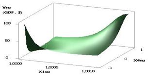
Fig. 1. V_su (GDP) = f(Х1, Х2, Х3, Х4)

Х1 = Х2 = Х3 = 1, Х4 = 0.99…–0.99

As the symmetrical Fig. 1 shows, the V_su (GDP) curve goes down at first to its minimum value V_su (GDP) = 5.25 units³ in the point 5 while the values of variable Х4 diminish, and further, with increase in negative values of X4, the plotted part of the V_su (GDP) curve mirrors the part of the curve with positive values of X4. This figure interprets the situation in a country in an economic crisis, when banks begin to lower key rates in an attempt to invigorate the economic situation. The calculations showed that the theoretical value of the V_su (GDP) under influence of external pressure, for example with Х4 = –0.99 equals V_sut (GDP) = 98.12. The volume of a spherical economic shell is calculated by using a formula V_su = 4pR_su³/3 = 4.19R_su³, units³. Thus, if the radius of a spherical economic shell R_su equals '1' (R_su = 1), we shall get V_su = 4.19 units³ calculating its volume V_su, i.e. less than the value of V_sut. Therefore, here we can introduce the notion of a singular volume of the spherical economic shell V_susv, i.e. when the value of V_susv = 1 units³. This is the starting value for every country's economy. In terms of our example, the theoretical value V_sut = 98.12 units³ with Х4 = 0.99, and V_sut = 5.23 units³ with X4 = 0.09, i.e. it decreased by a factor of 18,76 times, while the value of variable X4 is decreased by a factor of 11 times. Figure 1 leads to a conclusion that when a negative key rate is used, the V_su (GDP) of a country begins to grow.

Now we must mention that the calculated values of the amount of the V_su (GDP) depend on the accuracy we apply in calculating them. The value of the variable X4 greatly affects accuracy of the calculation, as shown in Table 1. This Table shows that along with increase in values of X4 from –0.9 to –0.999999, i.e. by a factor of 1.11111 times, the values of the GDP increase from 18.07 to 97756.52, i.e. by a factor of 5409.88 times.

Table 1. The combined table of values of X4 and of the Vsu (GDP) with values of X4 increasing
№	1.	2.	3.	4.	5.	6.
Value of X4	-0.9	-0.99	-0.999	-0.9999	-0.99999	-0.999999
Value of Vsu (GDP), units^3	18.07	98.12	549.93	3091.45	17383.90	97756.52

The similar Table 2 may be obtained when the values of the variable X4 decrease from –0.9 to –0.000009, i.e. by a factor of 100000 times, and the values of the V_su (GDP) decrease only by a factor of 3.48 times. In other words, it is safe to draw a conclusion here that if the values of the variable X4 decrease, the lower limit of the volume of economic shell of the V_su (GDP) may be assumed as 5.199.

Table 2. The combined table of values of X4 and of the Vsu (GDP) with values of X4 decreasing
№	1.	2.	3.	4.	5.	6.
Value of X4	-0.9	-0.09	-0.009	-0.0009	-0.00009	-0.000009
Value of Vsu (GDP), units^3	18.07	5.23	5.199	5.198982	5.1989792	5.1989791

On the basis of calculations presented in Tables 1 and 2 two curves have been plotted, shown on Fig. 2 and 3 respectively.

Fig. 2. Vsu (GDP) = f(Х1, Х2, Х3, Х4) Х1 = Х2 = Х3 = 1, Х4 = –0.9…–0.999999

Fig. 3. Vsu (GDP) = f(Х1, Х2, Х3, Х4) Х1 = Х2 = Х3 = 1, Х4 = –0.9…–0.000009

Additionally, the values of the V_su (GDP) for the curve plotted in Figure 2 may be calculated using a simpler formula by means of employing the following exponential equation of the V_su (GDP) = 3,178e^1,7211Х4, as the correlation coefficient R² in this case equals 1 (R² = 1).

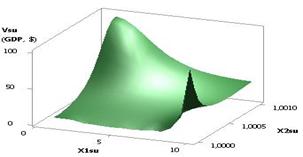
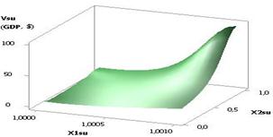
The following Figure 4 depicts a 3D graph for a 2D curve on Figure 1, which gives a more illustrative presentation of how a calculated parameter of the V_su (GDP) changes.

Fig. 4. V_su (GDP) = f(Х1, Х2, Х3, Х4)

Х1 = 1, Х2 = Х3 = 1, Х4 = 0.99…–0.99

In view of the fact that theoretical values V_sutmin > 0 and obviously diverge from practical values which can equal zero (V_supmin = 0), a diminution coefficient for K_sumin = 8.06E–11 can be introduced here. This coefficient helps render minimum theoretical values of V_sutmin into minimum practical V_supmin according to the formula V_sutmin = K_sumin V_supmin. Here we can offer a similar coefficient of increase for the maximum theoretical value of K_sumax which allows for rendering the maximum theoretical values V_sutmax into the maximum practical V_supmax according to the following formula V_sutmax = K_sumax V_supmax.

Table 3. The combined table of values of Х4 and maximum theoretical values of Vsutmax with values of Х4 increasing.
№	1.	2.	3.	4.	5.	6.
Value of Х4	-0.9	-0.99	-0.999	-0.9999	-0.99999	-0.999999
Value of Vsutmax, units^3	1.241	1.241	1.241	1.241	1.241	1.241

In the following two tables 3 and 4 there are the maximum theoretical values of V_sutmax, while values of the variable X4 increase and decrease. Table 3 shows that the values of V_sutmax, don't change and have the same amount of V_sutmax, = 1.241.

It can be seen from Table 4 that in the event of decrease in values of the variable Х4 from –0.9 to –0.000009, i.e. by a factor of 100000 times, the values of V_sutmax, decrease from 4.31 to 1.24080647, i.e. by a factor of 3.47 times.

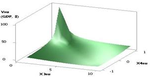
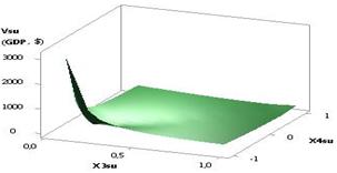
The following Figure 5 presents the V_su (GDP) curve with the following variables: Х1 = Х2 = 1, Х3 = 1…10, Х4 = 0.99…–0.99. As seen on the figure, the plotted curve plummets from 98.12 to 3.61 between the points 1 and 2, and continues to decrease to its minimum 0.3 in the point 8, and then increases to 3.1, i.e. by a factor of 10.31 times. Figure 6 below shows the same curve using 3D graph.

Table 4. The combined table of values of X4 and maximum theoretical values of Vsutmax with values of Х4 decreasing
№
Value of Х4	-0.9	-0.09	-0.009	-0.0009	-0.00009	-0.000009
Value of Vsutmax, units^3	4.31	1.24839	1.24088	1.240807	1.24080648	1.24080647

Fig. 5. Vsu (GDP) = f(Х1, Х2, Х3, Х4) Х1 = Х2 = 1, Х3 = 1…10, Х4 = 0.99…–0.99

Fig. 6. Vsu (GDP) = f(Х1, Х2, Х3, Х4) Х1 = Х2 = 1, Х3 = 1…10, Х4 = 0.99…–0.99

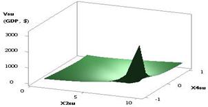
Further, in Figure 7 the V_su (GDP) dependency is illustrated with the variables Х1 = 1, Х2 = Х3 = 1…10, Х4 = 0.99…–0.99. It's noteworthy that the plotted curve has its minimum 28.85 in the point 2, and then the values of the V_su (GDP) grow to 3102.97, i.e. by a factor of 105.55. Now, if we compared the calculated values of the V_su (GDP), we would come up with the following values: with Х4 = 0.11 the values of the V_su (GDP) = 58.66, and with Х4 = –0.11 they jump to V_su (GDP) = 77.11. Thus, this option is acceptable in terms of economy's recovery from the crisis with the key rate having negative value. Figure 8 shows a three-dimensional picture of this curve.

Fig. 7. Vsu (GDP) = f(Х1, Х2, Х3, Х4) Х1 = 1, Х2 = Х3 = 1…10, Х4 = 0.99…–0.99

Fig. 8. Vsu (GDP) = f(Х1, Х2, Х3, Х4) Х1 = 1, Х2 = Х3 = 1…10, Х4 = 0.99…–0.99

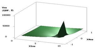
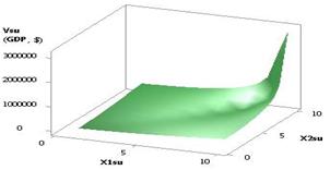
If all three first variables are increased by a factor of 10, Х1 = Х2 = Х3 = 1…10 with Х4 = 0.99…–0.99, then the values of the V_su (GDP) will be increased from 98.12 to a larger amount of the V_su (GDP) = 98124.68, i.e. by a factor of 1202.39, as shown in Figure 9. This option should be employed during a country's recovery from the economic crisis, as under any negative values of the variable Х4 the amount of the V_su (GDP) only grows. Here, the plotted curve has its minimum 81.62 in the point 2 and therefore the values of the variable Х1 = Х2 = Х3 = 2, Х4 = 0.77 shouldn't be applied. Figure 10 shows a three-dimensional picture of this dependency which in no way differs in appearance from the previous one in Figure 8.

Fig. 9. Vsu (GDP) = f(Х1, Х2, Х3, Х4) Х1 = Х2 = Х3 = 1…10, Х4 = 0.99…–0.99

Fig.10. Vsu (GDP) = f(Х1, Х2, Х3, Х4) Х1 = Х2 = Х3 = 1…10, Х4 = 0.99…–0.99

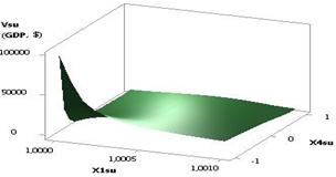
Fig. 11. Vsu (GDP) = f(Х1, Х2, Х3, Х4) Х1 = Х2 = 1…10, Х3 = 1, Х4 = 0.99…–0.99

Fig. 12. Vsu (GDP) = f(Х1, Х2, Х3, Х4) Х1 = Х2 = 1…10, Х3 = 1, Х4 = 0.99…–0.99

If we apply the following values of the variables Х1 = Х2 = 1…10, Х3 = 1, Х4 = 0.99…–0.99, the parameter V_su (GDP) will then be big too, increasing from 98.12 to 3.10E+06, i.e. by a factor of 31622.38 times, as shown in Figure 11. Therefore, this option is also recommended for use in selection of a way for a country's recovery from the crisis. Here, for example with Х4 = 0.11 the value V_su (GDP) = 7332.44, and with Х4 = -0.11, the V_su (GDP) will equal 16655.74, i.e. 2.3 times. Calculations served as a basis for a 3D graph, presented in Figure 12.

The following Figure 13 was plotted with Х1 = Х3 = 1, Х2 = 1…10, Х4 = 0.99…–0.99 and is analogous to Fig.9. As we can see here, the values of the V_su (GDP) do also reach a significant amount, from 98.12 they grow to 98124.68, i.e. by a factor of 1202.39 times. Here, the plotted curve has its minimum 81.62 in the point 2. Thus, the values of the variables where the V_su (GDP) = 81.62 shouldn't be selected during a country's recovery from the economic crisis. Figure 14 shows the influence two variables exert over the calculated amount of the V_su (GDP).

Fig. 13. Vsu (GDP) = f(Х1, Х2, Х3, Х4) Х1 = Х3 = 1, Х2 = 1…10, Х4 = 0.99…–0.99

Fig. 14. Vsu (GDP) = f(Х1, Х2, Х3, Х4) Х1 = Х3 = 1, Х2 = 1…10, Х4 = 0.99…–0.99

If we use the following values of the variables Х1 = Х3 = 1…10, Х2 = 1, Х4 = 0.99…–0.99 when we plot a curve of the V_su (GDP), we will get a curve presented in Fig.15, which is absolutely analogous to the curve in Fig.1. Therefore, here we can make the same conclusion. In Fig.16 below we see a three-dimensional interpretation of a two-dimensional graph in Fig.15.

Fig. 15. Vsu (GDP) = f(Х1, Х2, Х3, Х4) Х1 = Х3 = 1…10, Х2 = 1, Х4 = 0.99…–0.99

Fig. 16. Vsu (GDP) = f(Х1, Х2, Х3, Х4) Х1 = Х3 = 1…10, Х2 = 1, Х4 = 0.99…–0.99

Earlier, we had figures where the values of the variables Х1, Х2, Х3 grew by a factor of 10 times. Now we are going to look at the options where the variables Х1, Х2, Х3 will decrease, as illustrated in Fig.17 with Х1 = Х2 = 1, Х2 = 1…0.1. As the figure demonstrates, with the variable X3 decreasing by a factor of 10 times, the calculated values of the V_su (GDP) grow to the maximum value 3102.97, and the plotted curve has its minimum 9.52 in the point 3. Thus, this option is also suitable for a country's recovery from the economic crisis, excluding only the variables' values where the V_su (GDP) = 9.52. Figure 18 shows the 3D graph of the V_su (GDP).

Fig. 17. Vsu (GDP)= f(Х1, Х2, Х3, Х4) Х1 = Х2 = 1, Х2 = 1…0,1, Х4 = 0.99…–0.99

Fig. 18. Vsu (GDP) = f(Х1, Х2, Х3, Х4) Х1 = Х2 = 1, Х2 = 1…0,1, Х4 = 0.99…–0.99

If we calculate the parameter of the V_su (GDP) with the following values of the variables Х1 = 1, Х2 = Х2 = 1…0.1, Х4 = 0.99…–0.99, we will get a diminishing curve which has its minimum 0.91 in the point 9, and then grows to 3.1 in the point 10 (Fig.19). The obtained calculations served as a basis for a 3D graph, presented in Figure 20.

Fig. 19. Vsu (GDP) = f(Х1, Х2, Х3, Х4) Х1 = 1, Х2 =Х2 = 1…0,1, Х4 = 0.99…–0.99

Fig. 20. Vsu (GDP) = f(Х1, Х2, Х3, Х4) Х1 = 1, Х2 =Х2 = 1…0,1, Х4 = 0.99…–0.99

Fig. 21. Vsu (GDP) = f(Х1, Х2, Х3, Х4) Х1 = 1…10,Х2 = Х2 = 1…0,1, Х4 =0.99…–0.99

Fig. 22. Vsu (GDP)= f(Х1, Х2, Х3, Х4) Х1 = 1…10,Х2 = Х2 = 1…0,1, Х4 =0.99…–0.99

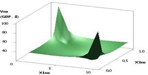
Figure 21 demonstrates that the plotted curve of the V_su (GDP) with Х1 = 1…10, Х2 = Х2 = 1…0.1, Х4 = 0.99…–0.99 imitates Fig. 1 and 15 by form and, naturally, the same conclusions also apply to it. It is noteworthy here that with these variables the minimum value of the V_su (GDP) equals 27.26. Figure 22 clearly demonstrates the look of this curve when its three-dimensional picture is used.

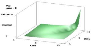
The last Figures 23 and 24 show 2D and 3D dependencies of the V_su (GDP) when the variables were the following: Х1 = Х2 = 1…10, Х2 = 1…0.1, Х4 = 0.99…–0.99. The calculations data show that with these variables the values of the V_su (GDP) were the biggest, increasing from 98.12 to 9.81E+07, i.e. grew by a factor of 1000000. This option is, thus, the most favourable for use in terms of recovery of a country's economy from the crisis.

Fig. 23. Vsu (GDP) = f(Х1, Х2, Х3, Х4) Х1 = Х2 = 1…10, Х2 = 1…0,1, Х4 = 0.99…–0.99

Fig. 24. Vsu (GDP) = f(Х1, Х2, Х3, Х4) Х1 = Х2 = 1…10, Х2 = 1…0,1, Х4 = 0.99…–0.99

We have the combined Table 5 below containing all the calculations referred to above. Their number is somewhat bigger as some parameters of the V_su (GDP) had both minimum and maximum values during calculations. Besides, all values of the V_su (GDP) parameters were sorted by a degree of diminution. Here, the values of V_sub and V_suf denote starting and ending values of the V_su (GDP) parameter, obtained by calculation. The ratio V_suf / V_sub characterises the extent of increase (decrease) of the last value of the parameter V_suf in relation to the starting V_sub. This enables us to single out such values of the variables Х1, Х2, Х3, Х4, where the V_su (GDP) grows even in the times of the economic crisis.

Table 5. Options of changing values of the variables X1 X2, X3 и X4, as well as calculated data Vsub and Vsuf and their ratio Vsuf / Vsub
№	Х1	Х2	Х3	Х4	Vsub…Vsuf (GDPsub… GDPsuf, $)	Vsuf / Vsub (GDPsuf / GDPsub)
1.	1…10	1…10	1…0.1	0.99…–0.99	98.12…9.81E+07	1.00E+06
2.	1…10	1…10	1	0.99…–0.99	98.12…3.10E+06	31622.78
3.	1…10	1…10	1…10	0.99…–0.99	81.61…98124.68	1202.39
4.	1	1…10	1	0.99…–0.99	81.61…98124.68	1202.39
5.	1	1	1…0.1	0.99…–0.99	9.52…3102.97	325.95
6.	1	1…10	1…10	0.99…–0.99	28.85…3102.97	107.55
7.	1	1	1	0.99…–0.99	5.24…98.12	18.70
8.	1…10	1	1…10	0.99…–0.99	5.25…98.12	18.70
9.	1	1	1…10	0.99…–0.99	0.30…3.10	10.31
10.	1…10	1…0.1	1…0.1	0.99…–0.99	24.63…98.12	3.98
11.	1	1…0.1	1…0.1	0.99…–0.99	0.91…3.10	3.40
12.	1…10	1…0.1	1…0.1	0.99…–0.99	24.63…27.26	1.11
13.	1…10	1…0.1	1…0.1	0.99…–0.99	27.26…24.63	0.90
14.	1…10	1…10	1…10	0.99…–0.99	98.12…81.61	0.83
15.	1	1…10	1	0.99…–0.99	98.12…81.61	0.83
16.	1	1…10	1…10	0.99…–0.99	98.12…28.85	0.29
17.	1…10	1…0.1	1…0.1	0.99…–0.99	98.12…24.63	0.25
18.	1	1	1…0.1	0.99…–0.99	98.12…9.52	0.097
19.	1	1	1	0.99…–0.99	98.12…5.24	0.05
20.	1…10	1	1…10	0.99…–0.99	98.12…5.25	0.05
21.	1	1…0.1	1…0.1	0.99…–0.99	98.12…0.91	0.009
22.	1	1	1…10	0.99…–0.99	98.12…0.30	0.003

The last table 6 is in fact a modified table 5, where only ratios V_suf / V_sub ≥ 1 are left. By doing so, we got the final Table 6 which combines all the values of the variables Х1, Х2, Х3, Х4, which can help us to drive the country out of the economic crisis. It's important to note here that an emphasis must be made during the selection of variables from Table 6 on those rows which have the maximum quantity of ones. In our example this happens with two values of the variables, highlighted in bold. In such case, only two variables should be changed, which is certainly easier than three or four.

Table 6. Options of changing values of the variables X1 X2, X3, X4, as well as calculated data Vsub and Vsuf and their ratio Vsuf / Vsub with Vsuf / Vsub ≥ 1
№	Х1	Х2	Х3	Х4	Vsub…Vsuf (GDPsub… GDPsuf, $)	Vsuf / Vsub (GDPsuf / GDPsub)
1.	1…10	1…10	1…0.1	0.99…–0.99	98.12…9.81E+07	1.00E+06
2.	1…10	1…10	1	0.99…–0.99	98.12…3.10E+06	31622.78
3.	1…10	1…10	1…10	0.99…–0.99	81.61…98124.68	1202.39
4.	1	1…10	1	0.99…–0.99	81.61…98124.68	1202.39
5.	1	1	1…0.1	0.99…–0.99	9.52…3102.97	325.95
6.	1	1…10	1…10	0.99…–0.99	28.85…3102.97	107.55
7.	1	1	1	0.99…–0.99	5.24…98.12	18.70
8.	1…10	1	1…10	0.99…–0.99	5.25…98.12	18.70
9.	1	1	1…10	0.99…–0.99	0.30…3.10	10.31
10.	1…10	1…0.1	1…0.1	0.99…–0.99	24.63…98.12	3.98
11.	1	1…0.1	1…0.1	0.99…–0.99	0.91…3.10	3.40
12.	1…10	1…0.1	1…0.1	0.99…–0.99	24.63…27.26	1.11

List of references:

1. Negative rates in mortgage. Now it's doable (in Russian).// http://www. vestifinance. ru/articles/52690

2. The Central Bank of Japan introduced a negative interest rate (in Russian) //https://news.mail.ru/ economics/24675278/

3. Negative interest rate (in Russian)// http://sverigesradio.se/sida/artikel.aspx? programid =2103&artikel=6091650

4. Negative interest rates (in Russian).// http://consulting-finance.com/stati/ otricatelnye-procentnye-stavki.html

5. Billions for charity: in Russia they won't understand that. The richest persons in the world Warren Buffet and Bill Gates offer the oligarchs to renounce their fortunes (in Russian). // https://svpressa.ru/world/article/26515/

6. The moneybags are asked to cede half of their wealth (in Russian). // http://www.mixnews.lv/ru/world /news/43138_boga4ej-prosyat-otdat-polovinu-nazhitogo/

7. Laura Keffer. Throughout 15 years in Russia 75% of the national income were moved to offshores (in Russian). // https://www.kommersant.ru/doc/3391074

8. Offshores in five graphs: trillions hidden from eyes of the beholder. // https://news.mail.ru/society/31625187/

9. The Russians hold 62 trillion roubles or 75% of the national income in offshores (in Russian). // https://newdaynews.ru/finance/612444.html

10. Olga Sorokina. Return to the motherland: how Russia handles deoffshorization of foreign assets (in Russian). // http://www.forbes.ru/biznes/336333-vozvrashchenie-na-rodinu-kak-rossiya-vedet-deofshorizaciyu-zarubezhnyh-aktivov