8.Математические
методы в экономике
Nickolay Zosimovich, Olga Kozhushko
National Aviation University, Institute of
International Relations (Kiev, Ukraine)
Modeling interbranch balance in a country with Leontief model
Summary. Analysis of the
sources on the task of input-output model was made by means of Mathcad with Leontief model. For a visual demonstration of the Leontief model, calculate balance for the state of Washington in 2002 (USA). Calculations show that if one of the indicators is large enough then the end result will be even higher.
Key words: economic
analysis,
balance, economic sector, industry, product, mathematical simulate, data, equilibrium, matrix, dynamic model, production
capacity.
I. Introduction.
The historical precursors to input-output
analysis were in evidence as far back as the first half of the XVII-th-century.
Most economic historians cite Francois Quesnay's (1694-1774) Tableau Economique
as the earliest recorded examples to depict the importance of mutual
interindustry flows or, in more modem parlance, systematic economic
interdependence (Addition 1). The model Quesnay created consisted of three economic movers [6]:
1. The “Proprietary” class, which consisted of just the landowners.
2. The “Productive” class, which contained all agricultural laborers.
3. The “Sterile” class, which contained artisans (craftsmen) and merchants.
The flow of production and/or cash between the three classes started with the
Proprietary class because they own the land and they buy from both of the other
classes. The process has these steps (Fig. 1):
1. The farmer produces 1500 food on land leased from the landlord. Of that
1500, he retains 600 food to feed himself, his livestock, and any laborers he
hires. He sells the remaining 900 in the market for $1 per unit of food. He
keeps $300 ($150 for himself, $150 for his laborer) to buy non-farm goods
(clothes, household goods, etc) from the merchants and artisans. This produces
$600 of net profit, to which Quesnay refers as product net.
2. The artisan produces 750 units of crafts. To produce at that level, he needs
300 units of food and 150 units of foreign goods. He also has subsistence need
of 150 units of food and 150 units of crafts to keep himself alive during the
year. The total is 450 units of food, 150 units of crafts, and 150 units of
foreign goods. He buys $450 of food from the farmer and $150 of goods from the
merchant, and he sells 600 units of crafts at the market for $600. Because the
artisan must use the cash he made selling his crafts to buy raw materials for
the next year’s production, he has not net profit.
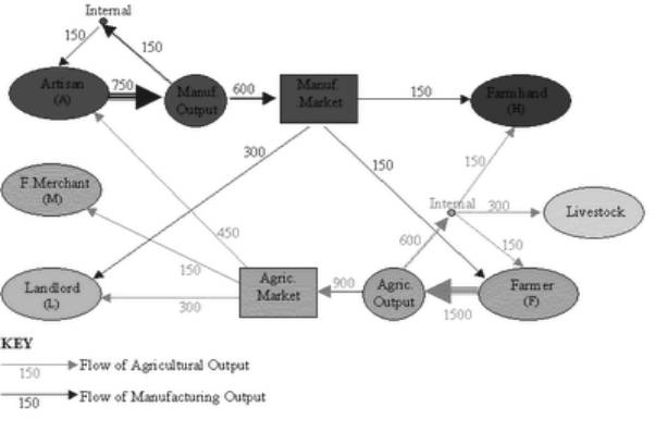
Fig. 1. Production Flow Diagram for Quesnay’s Tableau [6]
3. The landlord is only a consumer of food and crafts and produces no
product at all. His contribution to the production process is the lease of the
land the farmer uses, which costs $600 per year. The landlord uses $300 of the
rent to buy food from the farmer in the market and $300 to buy crafts from the artisan.
Because he is purely a consumer, Quesnay considers the landlord the prime mover
of economic activity. It is his desire to consume which causes him to expend
his entire lease income on food and crafts and which provides income to the
other classes.
4. The merchant is the mechanism for exporting food in exchange for foreign
imports. The merchant uses the $150 he received from the artisan to buy food
from the market, and it is assumed that he takes the food out of the country to
exchange it for more foreign goods [6].
II. Statement of the problem. Suppose an economy has n industries each producing a single unique
product. (There is a generalization of input output analysis, called activity analysis, in which an
industry may produce more than one product, some of which could be pollutants.)
Let the product input requirements per unit of product output be expressed as
an ![]() matrix A. Let X be
the n dimensional vector of outputs and F the n dimensional vector of final
demands. The amounts of production used up in producing output X is AX. This is
called the intermediary demand. The total demand is thus AX+F. The supply of
products is just the vector X. For an equilibrium between supply and demand the
following equations must be satisfied [2]:
matrix A. Let X be
the n dimensional vector of outputs and F the n dimensional vector of final
demands. The amounts of production used up in producing output X is AX. This is
called the intermediary demand. The total demand is thus AX+F. The supply of
products is just the vector X. For an equilibrium between supply and demand the
following equations must be satisfied [2]:
The equilibium production is then given by
A viable economy is one in which any vector of
nonnegative final demand induces a vector of nonnegative industrial
productions. In order for this to be true the elements of ![]() must all be positive. For this to be true
must all be positive. For this to be true ![]() has to satisfy
certain coditions.
has to satisfy
certain coditions.
A minor of a matrix is the value of a
determinant. The principal leading minors of an ![]() matrix are evaluated
on what is left after the last m rows and columes are deleted, where m runs
from (n-1) down to 0.
matrix are evaluated
on what is left after the last m rows and columes are deleted, where m runs
from (n-1) down to 0.
The condition for the ![]() matrix of
matrix of ![]() to have an
inverse of nonnegative elements is that its principal leading minors be
positive. This is known as the Hawkins-Simon conditions [2].
to have an
inverse of nonnegative elements is that its principal leading minors be
positive. This is known as the Hawkins-Simon conditions [2].
Synthesizing knowledge about reproduction theory of
Marx and Engels, cybernetics, Norbert Wiener and the economic and mathematical
model of input-output balance (IOB) Leontief, as well as a huge personal
experience as a mechanical engineer and an organizer of production at different
levels of management corporation of the USSR, the creator of the first
Automated Control Systems (ACS), founder of the school strategic planning
Veduta Nikolai Ivanovich (1913-1998) developed a dynamic model of the IOB which
suggests the inclusion of the impact of the market
(equilibrium prices) to determine the proportions of the plan.
In the scheme of IOB for the first time systematically
coordinated balance of revenues and outlays of producers and consumers - the
state (inter-state block), households, exporters and importers (the external
economic balance). A dynamic model of IOB his method of economic cybernetics.
It is a system of algorithms, effectively linking the tasks of end users with
capabilities (material, human and financial), producers of all forms of
ownership. Based on the model is determined by the effective allocation of
productive government investment. Introducing a dynamic model of IOB, the
government is able to adjust the mode «online» for development based on
refinement of the production capacity of residents and demand dynamics of end
users to meet the requirements of national and global security [3].
III. Simulation methodics of Leontief model. For a visual demonstration of the Leontief model, calculate balance for the state of Washington. From the "input-output" table of Washington in 2002 [1] choose the input data for calculations (Table 1).
Table 1
The input data for task
|
|
Mining |
Electric Utilities |
Gas Utilities |
Air Transportation |
Inter-industry subtotal |
Total final demand |
|
Mining |
0,8 |
124,8
|
14,2
|
0,0 |
139,8 |
139 |
|
Electric Utilities |
10,5
|
1773,0 |
0,4 |
3,2 |
1787,1 |
14,1 |
|
Gas Utilities |
2,8 |
134,1
|
1,0 |
0,3 |
138,2 |
137,2 |
|
Air Transportation |
0,2 |
5,6 |
0,7 |
0,2 |
6,7 |
6,5 |
|
Total
intermediate input |
14,3 |
2037,5 |
16,3 |
3,7 |
2071,8 |
|
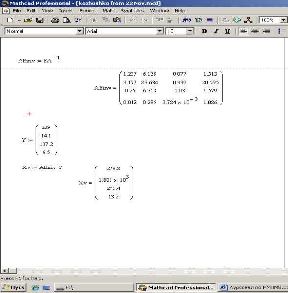
Fig. 2. Results of Table 1
calculation
For the final demand
Y=(139;14,1;137,2;6,5) total output for Mining is 278,8, Electric Utilities – 1.801х103
, Gas Utilities – 275,4, Air Transportation – 132 (Fig. 2). Because of too much the end
result of Electric Utilities, reduce
its input rate by 2 times and then change the vector of final demand
(Table 2).
Table 2
A modified input data for task
|
|
Mining |
Electric Utilities |
Gas Utilities |
Air Transportation |
Inter-industry subtotal |
Total final demand |
|
Mining |
0,8 |
124,8
|
14,2
|
0,0 |
139,8 |
139 |
|
Electric Utilities |
10,5
|
886,5 |
0,4 |
3,2 |
1787,1 |
900,6 |
|
Gas Utilities |
2,8 |
134,1
|
1,0 |
0,3 |
138,2 |
137,2 |
|
Air Transportation |
0,2 |
5,6 |
0,7 |
0,2 |
6,7 |
6,5 |
|
Total
intermediate input |
14,3 |
2037,5 |
16,3 |
3,7 |
2071,8 |
|
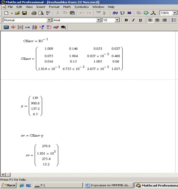
Fig. 3. Results of Table 2
calculation
Repeating calculation with a
reduced rate Electric Utilities 2 times showed
that this significant reduction caused a small variation of
certain parameters, but the end result is not affected. It means that for the final demand Y=(139;900,6;137,2;6,5) total output is the same: Mining – 278,8, Electric Utilities – 1.801х103
, Gas Utilities – 275,4, Air Transportation – 132 (Fig. 3).
IV. Conclusions. Leontief model has a strong historical background which shows that interest in the issue of interbranch relations in the economy concerned scientists for many years.
1. There are related methods that specify the calculations and give a more accurate result.
2. Leontief model is very useful because it includes the important factors that significantly affect the economy as a
whole.
3. Calculations show that if one of the indicators is large enough then the end result will be even higher.
4. If this indicator reduce significantly the end result does not change. In the
calculation process certain parameters change only.
The calculations produced above have a illustrative
purpose. In order to trace the significant changes and get more specific and accurate results it is necessary to make
a matrix which will include a greater number of industries. Here it
is necessary to change indicators separately to follow the trend. In practice use an additional parameters such as value
added, imports, total employment etc.
References
1.
http://www.ofm.wa.gov/economy/io/2002/default.asp
- Office of Financial Management.
2.
http://www.sjsu.edu/faculty/watkins/inputoutput.htm#INTRO
- San José State University
Department of Economics.
3.
http://ru.wikipedia.org/wiki/ - Межотраслевой_баланс.
4. http://en.wikipedia.org/wiki/Tableau_%C3%A9
– economique.
5. http://www.referenceforbusiness.com/encyclopedia/Inc-Int/Input-Output-Analysis.html
- Reference for Business. Encyclopedia
of Business, 2nd ed.
6.
http://econ-thought.blogspot.com/2010/01/francois-quesnays-tableau-economique.html
- Modern Economic Thought.