NEW METHODS OF
APPROXIMATION OF PIECEWISE
LINEAR FUNCTIONS
Piecewise functions are widely
applied in various areas of scientific research. Technical and mathematical
disciplines, such as automatic control theory, electrical and radio
engineering, information and signal transmission theory, equations of
mathematical physics, theory of vibrations, and differential equations are
traditional fields of application [1–3].
Systems with piecewise parameters
and functions are considered highly nonlinear structures to emphasize the
complexity of obtaining solutions for such structures. Despite the simplicity
of piecewise functions in segments, the construction of solutions in problems
with piecewise functions on the whole domain of definition requires using
special mathematical methods, such as the alignment method [4] with the
coordination of the solution by segments and switching surfaces. Generally,
application of the alignment method requires overcoming substantial
mathematical difficulties, and intricate solutions represented by complex
expressions are obtained rather often.
In many cases, researchers
rely upon approximation methods using Fourier series  , where
 ![]() is an orthogonal system in functional Hilbert
space
is an orthogonal system in functional Hilbert
space ![]() of measurable functions with Lebesgue
integrable squares,
of measurable functions with Lebesgue
integrable squares, ![]() . The trigonometric system of
. The trigonometric system of ![]() ─ periodic functions
─ periodic functions ![]() is often taken as an orthogonal system. In this
case, the following is fulfilled in the vicinity of discontinuity points
is often taken as an orthogonal system. In this
case, the following is fulfilled in the vicinity of discontinuity points ![]()
![]() , where
, where ![]() is the partial sum of the Fourier series. It is
how Gibbs’ phenomenon shows itself [5]. Thus, in the case of a function
is the partial sum of the Fourier series. It is
how Gibbs’ phenomenon shows itself [5]. Thus, in the case of a function
![]() (1)
(1)
the point ![]() , where
, where ![]() is the integral part of the
number
is the integral part of the
number![]() , is the maximum point of the partial sum
, is the maximum point of the partial sum ![]() of the trigonometric Fourier
series [5] with
of the trigonometric Fourier
series [5] with  , i.e., the absolute
error value is
, i.e., the absolute
error value is ![]() . It should be noted
that
. It should be noted
that ![]() .
.
The graph of the partial sum ![]() of the trigonometric series on the interval
of the trigonometric series on the interval ![]() , which illustrates the presence of the Gibbs phenomenon is presented in
Fig. 1.
, which illustrates the presence of the Gibbs phenomenon is presented in
Fig. 1.
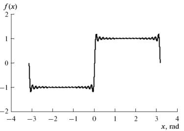
Fig. 1. Presence of
the Gibbs phenomenon
What is unpleasant in this
case is that the Gibbs effect is generic and is present for any function ![]() , which has limited variation on the interval
, which has limited variation on the interval ![]() , with isolated discontinuity point
, with isolated discontinuity point ![]() . The presence of the Gibbs phenomenon leads to extremely negative
consequences of the use of the partial sum of a trigonometric series as an
approximating function in fields such as radio engineering and signal
transmission.
. The presence of the Gibbs phenomenon leads to extremely negative
consequences of the use of the partial sum of a trigonometric series as an
approximating function in fields such as radio engineering and signal
transmission.
In order to eliminate the
mentioned disadvantages, new methods of approximation of piecewise functions
based on the use of trigonometric expressions represented by recursive
functions were suggested in the paper [6] and developed in this report.
For example, consider the piecewise
function (1) in more detail. This function is often used as an example of the
application of Fourier series, and, therefore, it is convenient to take this
function for comparative analysis of a traditional Fourier series expansion and
the suggested method. Expansion of (1) into Fourier series has all the above
mentioned disadvantages. In order to eliminate them, it is proposed to
approximate the initial step function by a sequence of recursive periodic
functions
![]() (2)
(2)
Graphs of the initial function
(a thickened line) and its five successive approximations for this case are presented
in Fig. 2. It can be seen that, even when n values are relatively small
in the iterative procedure (2), the graph of the approximating functions
approximates the initial function (1) rather well. In addition, approximating
functions obtained using the suggested methods do not have any of the
disadvantages of Fourier series expansion. There is absolutely no sign of the
Gibbs phenomenon.
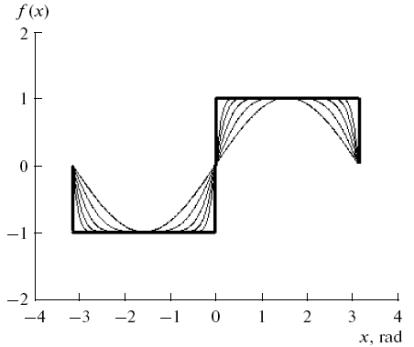
Fig. 2. Graphs of the initial
function and its five successive approximations
The number ![]() was used in the sequence of approximating
functions (2) as a constant factor; however, it is possible to take another
factor, which may be variable as well. Cosine and other trigonometric functions
and their combinations may be used instead of sine in the suggested method of
approximation. For example,
if we use the sequence of recursive functions
was used in the sequence of approximating
functions (2) as a constant factor; however, it is possible to take another
factor, which may be variable as well. Cosine and other trigonometric functions
and their combinations may be used instead of sine in the suggested method of
approximation. For example,
if we use the sequence of recursive functions
![]() ,
,
we may approximate short-term impulses. The graph of one function from
such sequence is presented in Fig. 3.
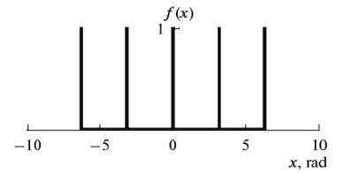
Fig. 3. Graph of the
analytical function that approximates short-term pulses
In some cases for more
precise approximation of the initial function by means of the suggested methods it does not make sense to bring the approximating function to the position
close to the limit. It may appear
that the optimal approximation
occupies an intermediate position between
the two neighboring approximation members ![]() and
and ![]() of the sequence of
recursive functions (2). In such
cases, the approximating function can be written as
of the sequence of
recursive functions (2). In such
cases, the approximating function can be written as ![]() , where
, where ![]() . As an illustration for such
cases it may serve graphs in Fig. 4. Here curve 1 corresponds to the function
. As an illustration for such
cases it may serve graphs in Fig. 4. Here curve 1 corresponds to the function ![]() , curve 2 ─ the function
, curve 2 ─ the function ![]() . Dashed line 3
corresponds to an intermediate function
. Dashed line 3
corresponds to an intermediate function
![]() .
.
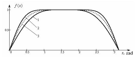
Fig. 4.
1 2 3
Construction of an intermediate approximation functions
The suggested methods of approximation by
a sequence of recursive functions
(2) can be used not only for the step
functions, but for piecewise linear
functions in general, which greatly expands the scope of the
considered approximate procedures.
For example, let us consider the following piecewise linear
function
 (3)
(3)
Here we have ![]()
Taking the continuity of the function in![]() into consideration, we can find
into consideration, we can find ![]() .
.
Let ![]() , then the frequency factor
, then the frequency factor ![]() for the
approximating function can be calculated by the formula
for the
approximating function can be calculated by the formula ![]() , where
, where![]() .
.
Let us introduce some notations ![]() . Then the approximating function
for piecewise linear function (3)
can be constructed by such way
. Then the approximating function
for piecewise linear function (3)
can be constructed by such way
![]() .
.
For the function  the approximation function
will be
the approximation function
will be ![]() . Graphs of these functions,
constructed with the help of a computer
program, are shown in Fig. 5.
The graph of the initial
function is built using the logical operator
. Graphs of these functions,
constructed with the help of a computer
program, are shown in Fig. 5.
The graph of the initial
function is built using the logical operator ![]() , which in our case takes the form
, which in our case takes the form ![]() . We can
see that the graphics of the initial piecewise function and its approximation in a given scale are completely fused.
. We can
see that the graphics of the initial piecewise function and its approximation in a given scale are completely fused.
Moreover, by using the suggested procedure
not only piecewise linear continuous functions, but piecewise linear
function with non-removable discontinuities of the first kind can be
approximated. For example, in Fig. 6 the graph of the function  (the thick line) and its
approximation
(the thick line) and its
approximation ![]() (the thin line), where
(the thin line), where ![]() , are given.
, are given.
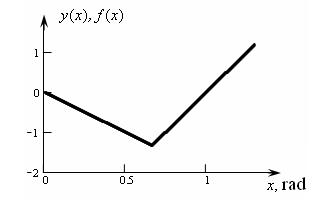
Fig. 5. Graphs of the piecewise function and its approximations
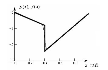
Fig. 6. The example of approximation of a discontinuous piecewise
linear function
The approximation error can be arbitrarily
small by increasing the number of
nested trigonometric functions in the approximating function. Besides, note that the number of points of discontinuities of a piecewise linear
functions has essentially no effect on
the possibility of approximating these
functions by suggested methods.
REFERENCES
1. A. V. Nikitin and V. F. Shishlakov, Parametric Synthesis of Nonlinear Automatic Control Systems, (SPbGUAP,
St. Petersburg, 2003) [in Russian].
2. D. Meltzer, “On the Expressibility of Piecewise Linear Continuous
Functions as the Difference of Two Piecewise Linear Convex Functions,” Math.
Program., Study 29, 118–134
(1986).
3. S. I. Baskakov, Radio
Engineering Chains and Signals: Textbook for Higher_Education Institutions.,
3rd ed. Vysshaya shkola, Moscow, 2000) [in Russian].
4. E. P. Popov, Theory of
Nonlinear Automatic Regulation and Control Systems: Textbook, 2nd ed.
(Nauka. Gl. red. fiz.-mat. lit, Moscow, 1988) [in Russian].
5. G. Helmberg, “The Gibbs Phenomenon for Fourier Interpolation,” J.
Approx. Theory 78, 41–63 (1994).
6. S. V. Alyukov, “Approximation
of Step Functions in Problems of Mathematical Modeling,” Mathematical
Models and Computer Simulations, 2011, Vol. 3, No. 5, pp. 661–669. © Pleiades
Publishing, Ltd., 2011. Original Russian Text © S.V. Alyukov, 2011, published
in Matematicheskoe Modelirovanie, 2011, Vol. 23, No. 3, pp. 75–88.