Tехнические науки/ Авиация и космонавтика

Nickolay Zosimovych¹, Anatoly Voytsytskyy²

¹Tecnólogico de Monterrey (Campus Gualajara, Mexico)

²Zhytomyr National Agrarian and Ecological University (Zhytomyr, Ukraine)

DISTURBED MOTION OF THE LAUNCH VEHICLE WITH INTEGRATED GPS/INS NAVIGATION SYSTEMS

In these article has been conducted a presimulation analysis of disturbed motion of the launch vehicle with integrated GPS/INS navigation systems. It was determined the main characteristics describing the internal structure of vehicle.

Key words: Integrated GPS/INS navigation systems, gimbaled inertial navigation system (GINS), GPS receiver, launch vehicle, mathematical model (MM), thrust, propulsion, deviation.

Introduction. A key tendency in the development of affordable modern navigation systems is displayed by the use of integrated GPS/INS navigation systems consisting of a gimbaled inertial navigation system (GINS) and a multichannel GPS receiver [1]. The investigations show [2, 3], that such systems of navigation sensors with their relatively low cost are able to provide the required accuracy of navigation for a wide class of highly maneuverable objects, such as airplanes, helicopters, airborne precision-guided weapons, spacecraft, launch vehicles and recoverable orbital carriers.

Let us briefly examine the scientific and technical problems arising when making the corresponding models and algorithms.

MM of spatial motion of center of mass and relative to center of mass of a solid launch vehicle is well known and widely described in sources. The greatest difficulty in the implementation of such a model as a part of the model of the environment, represents a model of a solid-propellant rocket engine with thrust distribution in respect to the nominal model in mind and the model of stage separation from the point of view of the influence of disturbing moments that arise when dividing into initial conditions of the motion of the next stage.

Task Statement. Let's consider the above objectives, having regard to peculiarities of the subject of inquiry, namely a commercial launch vehicle, designed to launch payloads into low Earth orbit (LEO) or geostationary orbit (GSO), in more details.

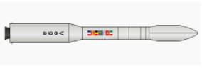
Fig. 1. Launch vehicle Vega (Vettore Europeo di Generazione Avanzata, ASI&ESA) [4]

Within the framework of this study we shall consider a light launch vehicle which has been jointly developed by the European Space Agency (ESA) and the Italian Space Agency (ASI) since 1998 (Fig.1). It is qualified to launch satellites ranging from 300 kg to 2000 kg into low circular polar orbits. As a rule, these are low cost projects conducted by research organizations and universities monitoring the Earth in scientific missions as well as spy satellites, scientific and amateur satellites. The launch vehicle Vega [4] is the prototype of the vehicle under development.

The planned payload to be delivered by the launch vehicle to a polar orbit at an altitude of ~700 km shall be 1500 kg. The launch vehicle is tailored for missions to low Earth and Sun-synchronous orbits. During the first mission the light class launch vehicle is to launch the main payload, a satellite weighing 400 kg, to an altitude of 1450 km with an inclination of the orbit 71.50⁰. Unlike most single-body launchers, this vehicle is to launch several spacecraft.

In order to make a model for disturbed motion of the above mathematical model shall be supplemented with mathematical models of the following disturbing factors:

· thrust distribution in the propulsion system in respect to nominal thrust profile;

· manufacturing defects of structure and assembly components;

· variations of atmospheric parameters and wind fields.

Let's cconsider a model of each of these factors in detail.

A model of thrust distribution in the propulsion system. As mentioned above, nominal profiles of thrust in vacuum and the nominal mass flow rate of the propellant specified in a table are used when calculating a thrust. In addition to the nominal profile of thrust and propellant mass flow the performance of propulsion system accompanies the product with profiles of the so-called "upper" and "lower" thrust with relevant profiles of propellant mass flow and of the center of gravity of the fuel solid-block (Fig.2).

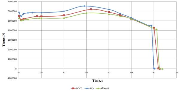
Fig. 2. Profiles of propellant mass flow

These profiles characterize variation of the burning rate of the fuel solid-block depending on the specific chemical composition of the propellant, atmospheric conditions, location of the fuel solid-block inside the propulsion system, etc.

In order to make a model of thrust distribution we may apply deterministic, stochastic and minimax approaches. Proceeding from the physical aspect of the factor discussed we applied the stochastic approach in this paper [5] based on the following.

The distribution of thrust was considered as a uniformly distributed random variable in the range with -1 corresponding to the "lower" thrust, 0 being the nominal profile and +1 being the "upper" thrust. This random variable is implemented for each engine of the launch vehicle only one time before the simulation hereafter the profile of real thrust as well as of mass consumption and of the center of the fuel solid-block shall be constructed based on the Chebyshev polynomials approximation and used similarly as in the calculation of traction, weight and control moments of the launch vehicle.

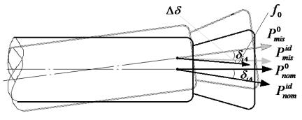
Fig. 3. Engine deviations and deflection angles of the nozzles in development tests (failure tests) of control inputs: is a sum of forces acting upon the launch vehicle; is an ideal nominal thrust of the propulsion system; is nominal thrust of the propulsion system in vacuum environment; is a «disturbed» ideal thrust; is «disturbed» thrust in vacuum environment; is engine «deviation» of the launch vehicle; is deflection angle of the nozzles consequent on testing and correction of control signals

The line of thrust shall be determined in the body-fixed frame and depend on the orientation of the longitudinal axis of the nozzle relative to the longitudinal axis of the launcher engine. When considering the undisturbed motion of the launch vehicle, engine angles shall be regarded as nominal and the direction is determined only by the deflection angles of the nozzles consequent on testing and correction of control signals (Fig. 3). When considering the disturbed motion of the launch vehicle, the line of thrust shall be determined on account of errors in the assembly of the launch vehicle, engine deviations and errors in testing and correction of controlling influence. Let's consider errors in the assembly of the launch vehicle and engine deviations closer.

Manufacture defects of structure and assembly components of the launch vehicle. As already mentioned, when considering the undisturbed motion the launch vehicle shall be considered as ideally assembled, i.e. axes of the structure members coinсide, there is no displacement between the members, etc. In a real situation assembly errors are inevitable along reasonable length of the launch vehicle which leads to a change in the moments of inertia of the launch vehicle, the center of mass, and most importantly, a change in the thrust line.

To describe this disturbing factor let's consider the launch vehicle as a combination of components that make it up (a nose cone, a satellite with a bus, the fourth stage engine pack, a control bay, the third stage block, the second stage block, the first stage boosters) [5]. Each of these components has its mass and inertial characteristics (depending on the change in its mass. The moment of inertia, the center of block mass are set by designers of the launch vehicle) in an ideally bound coordinate system.

In addition, each component is characterized by the coordinates of points of its anchorage with the adjacent components and assembly errors, given in the form of the tilt -related coordinate system relative to the adjacent structural component [5]. This error is considered normally expected corresponding to the nominal arrangement of components and variance set by designers of the launch vehicle [6] (Fig. 4).

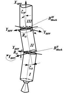
Fig. 4. Errors in the assembly of stages in a bound coordinate system

So, for example, errors in the assembly of the third stage block relative the control unit are characterized by incidental orientation angles.

Usually assembly begins with the control unit because it includes a measuring unit and a gyroplatform implementing inertial reference frame and measuring the orientation angles of the launch vehicle [5]. Further units shall be docked up and down the launch vehicle subject to specific error values in the assembly of the launch vehicle. Thus, the center of mass and moments of inertia shall be recalculated in the bound reference frame. Besides, there shall be calculated deflection angles of the nozzles of the launch vehicle and arms of thrust forces required in the calculation of moments.

A model of variations of atmospheric parameters and wind fields. As is known, the aerodynamic forces acting on the launch vehicle are in particular dependent on the atmospheric parameters (density, pressure, temperature). These parameters, in their turn, depend on the altitude and geographic latitude, time and season, the parameters of solar activity and other factors.

To calculate trajectories and conduct other studies we should use standard atmosphere (SA) tables while designing a launch vehicle. They give some average parameters for tranquil atmosphere depending on the height [6-8]. Deviations of the atmospheric parameters from the standard values, as well as wind are atmospheric disturbances which are taken into consideration when one studies the disturbed motion of the launch vehicle.

To solve the problems of flight dynamics, we also need to know the range of possible deviations of these parameters corresponding to a certain level of probability in addition to standard values of atmospheric parameters both excluding seasons and locations on the globe, and taking them into account. In addition, more accurate research requires knowledge of the statistical relationships between the random deviations of each parameter at different heights, etc.

There are various methods describing disturbance of atmospheric parameters. In the present paper, we shall use the canonical expansion method for random components of atmospheric parameters [9]. The substance of the method is as follows. The temperature and the density of the atmosphere can be represented in the following way [10]:

where are standard values of the temperature and the density ;

is deviation from the standard temperature;

is a relative deviation from the standard air density.

In order to set random functions and we shall use the canonical expansion method [11].

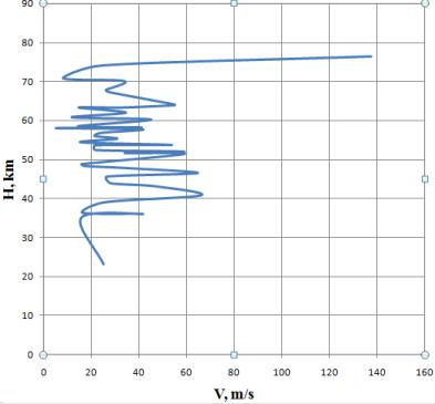
Fig. 5. Mean values of the zonal wind component in Guam (processing of the results by the author based upon the data obtained by 9 meteorological rockets during the period between 3rd and 25th September, 1958) [12]

With reference to the case under consideration, the atmospheric parameters as random functions of height of a point above the Earth's surface are represented as canonical expansion as follows:

where are mean deviations from the values of standard atmosphere corresponding to the point in question;

are some nonrandom deviation from the mean deviations and

Wind effect is taken into account in changing airspeed vector. Thus, taking into account the effects of wind air vector shall be written as:

where is an air vector in undisturbed motion; is a gust velocity vector.

Wind shall be considered horizontal, i.e. without vertical movement of air masses, and the absolute velocity depends on the altitude and geographical coordinates of the point, and the direction is characterized by azimuth angle - i.e. wind direction relative to the north.

The absolute value of the wind speed is determined by approximating of the profiles of wind velocity that are set apriori (Fig. 5), and the azimuth angle is a random variable normally distributed with mean corresponding to the nominal direction of the wind variance given by the Customer:

CONCLUSIONS

1. Based on the above, we have set a technical problem of the conceptual design of an integrated navigation system for the space launch vehicle qualified to inject small artificial Earth satellites into low and medium circular orbits.

2. We have made an analysis of possible models of flight and navigation measurements and identified key potential difficulties in the process of their creation.

References

1. Zosimovych Nickolay. Integrated Navigation System for Prompting of the Commersial Carrier Rocket. Information technology Conference for Academia and Professionals (ITC-AP 2013), Sharda University, India, 19-21 April, 2013.

2. Flight instruments and navigation systems. Politecnico di Milano - Dipartimento di Ingegneria Aerospaziale, Aircraft systems (lecture notes), version 2004.

3. George M. Siouris. Aerospace Avionics Systems. Academic Press, INC 1993.

4. http://ru.wikipedia.org/wiki/ - Вега (ракета-носитель).

5. Veniamin V. Malyshev, Michail N. Krasilshikov, Vladimir T. Bobronnikov, Victor D. Dishel. Aerospace vehicle control, Moscow, 1996.

6. Furman T.T. Approximate Methods in Engineering Design, Vol. 155: Mathematics in Science and Engineering, Edited by Richard Bellman, 1981.

7. CIRA 1972 (COSPAR International Reference Atmosphere 1972), Berlin, 1972.

8. ГОСТ 4401-64. Таблицы стандартной атмосферы. Изд-во стандартов, Москва, 1964.

9. Carlo L. Botasso. Solution Procedures for Maneuvering Multibody Dynamics Problems for Vehicle Models of Varying Complexity. Multibody Dynamics, Computational Methods in Applied Sciences, Vol. 12, pp.57-79, 2008.

10. Steven A. Hildereth, Carl Ek. Long-Range Ballistic Missile Defence in Europe. Congressional Research Service, RL34051, January 21, 2009.

11. Albertos P., and Sala A. Multivariable Control Systems, Valensia, Spain, 2004.

12. Матвеев Л.Т. Основы общей метеорологии. Физика атмосферы. Л.: Гидрометеоиздат, 1965, 867 с.