Математика/4. Прикладная
математика
Plekhanov N.S.
Murom Institute of
Vladimir State University, Murom, Russia
An overview and analysis of the
thinning algorithms
1. INTRO
Owing to the discrete nature of binary images, skeleton models have to be
adapted in a discrete context. Discrete distances will help in measurements, whereas
connectivity will prove fundamental for developing and evaluating these
algorithms. The aim is to characterize a skeleton as a set of pixels S within the
foreground of the original image. In this paper, discrete equivalents to the
models presented are found and described.
These
techniques can be divided into two main categories. The first class of techniques,
referred to as skeletonisation techniques, first characterize a set of "skeletal"
pixels eligible to belong to the final skeleton.
The
algorithms of the second class are called thinning algorithms and process the image
iteratively until the skeleton set S is obtained.
In
Section 2, classical algorithm which relies heavily on discrete distances and distance
maps is presented. This algorithm belongs to the class of skeletonisation algorithms
since it first characterizes a skeletal set which is then post-processed. Section
3 then proposes to use the well-structured context of mathematical morphology to
perform thinning. The most commonly used operators are defined and their implementation
discussed. As a complement, a different approach which is based on the
minimum-base segment algorithm is presented in Section 4.
2. CENTRES OF MAXIMAL DISCS
This
approach relies on Blum's model of a binary component F. The idea behind this technique
is to characterize a set of skeletal pixels (i.e. eligible for being skeleton pixels)
as the set of centers of maximal discs in the component. The skeletal set is then
processed. In particular, connectivity and one-pixel width are ensured via deletion
or addition of pixels in this set.
The
use of a specific discrete distance dD has first to be decided. It is commonly admitted
that chamfer distances allow for an efficient characterization of the centers of
maximal discs. We should noted that the value of the distance transformation of
F at p, DTD (p), indicates the radius of the largest discrete disc centered at p
and totally contained in F. Combining this result, centers of maximal discs in F
can clearly be characterized as pixels in F which correspond to local maxima in
the distance map of F.
Strictly
speaking, centers of maximal discs are local maxima of the distance map if and only
if the basic move length (i.e. a) is 1. When extending discrete distances, this
property is lost but the name is kept.
When
using discrete distances, a pixel q E F participates in the propagation of the distance
transformation value from a border pixel r to a pixel p (neighbour of q) if and
only if DTD(p) - DTD(q) + do(p, q), where DTD(q) - dD(q, r). A pixel is a centre
of maximal disc if it does not participate in the propagation of the distance transformation
value at any pixel. In summary, the following proposition holds.
By
definition, a centre of maximal disc is a pixel located on the ridge of the
scalar field created by the distance map. At a centre of maximal disc, border
influence therefore switches from one side to the opposite. By duality, considering
borders as generators of a generalized Voronoi diagram, the set of centers of
maximal discs therefore constitute the borders of Voronoi cells. Figure 1 shows
an example of a binary image and its associated distance map.
In
this representation, each pixel is connected to its closest border pixel. White
like areas corresponding to ridges in the distance map show locations of centers
of maximal discs and constitute edges of the Voronoi diagram. By definition they
also form the skeleton of this binary component.
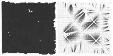
Figure
1 - Discrete Voronoi diagram deduced from the distance map
Depending
on the application considered (e.g. compression or representation), the skeletal
set may be post-processed in different ways to emphasize different conditions.
If
thinning is performed with the aim of representation, some pixels are therefore
to be removed or added in the skeletal set to form the final skeleton. Such
post-processing mostly relies on the inspection of the neighbourhood of each
pixel in the skeletal set. The use of connectivity and crossing numbers then helps
in deciding whether to add (or remove) a specific pixel to (or from) the skeletal
pixel. More generally, the definition of neighbourhood masks (i.e. templates)
which show allowed and forbidden patterns in the skeletal set allows for respecting
specific constraints. This is formally described, next, using a morphological approach.
As
further processing, a pruning process will remove small branches from the skeletal
set, considered as spurious. In this respect, such step is often called a "beautifying
step".
When
the aim of thinning is compact storage (i.e. compression), redundancy has to be
removed from the skeletal set. The skeletal set as it is given above allows for
exact (complete) reconstruction of the original image. However, a subset may be
defined such that it still allows for exact reconstruction while including fewer
pixels (e.g. see [1, 2, 3]).
3. MORPHOLOGICAL APPROACH
When using a morphological approach, thinning is related to the wave
propagation model proposed earlier. In the discrete space (i.e. using pixels), wave
fronts are propagated. In this section, we simply introduce the concepts related
to morphological skeletons and morphological thinning. For a thorough study of
morphological thinning and skeletons, the reader is referred to [4, 5, 6, 7].
Morphological skeleton
Let F be the foreground of a binary image. The morphological skeleton S of
F is defined by

where
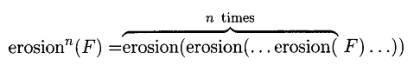
![]()
The notation erosionn (F) denotes n successive applications of
the erosion(.) operator to F:
By definition of Fn, the union is clearly reduced to

where N is the smallest integer value such that FN+ 1 = 0.
Let’s see an example of morphological skeletonisation of a simple binary
image (Figure 2). Here, ND = N4.
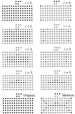
Figure 2 - Morphological skeleton
The left column shows successive sets Fn and the right column
shows successive sets Sn. In that case N = 3 since F4 = 0.
The bottom row compares F and S. Note that, in this case, S is a disconnected set.
Use of the definition of a morphological skeleton in its digitized form may
result in a disconnected skeleton set S even if the original component F is connected.
Therefore, the definition of a morphological thinning operator has been introduced.
4. MINIMUM-BASE SEGMENT ALGORITHM
In the discrete space, skeletonisation based on local width simply uses pixels
as border points and follows the borders of the component in directions allowed
by the connectivity relationship given in the current context. The algorithm
shows some shortcomings which are overcome in [8].
The main advantage of such a discrete approach is that it creates pairs of
border pixels to form local width lines. These lines have been shown to be
optimal for local width measurements and therefore for analyzing the image. An example
is illustrated in Figure 3 where the skeleton and dual width lines are shown for
a ribbon-like image.
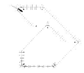
Figure 3 - Skeleton and local width measurement
REFERENCES
1. J. Goutsias and D. Schonfeld. Morphological representation of
discrete and binary images. IEEE Transactions on Signal Processing,
39(6):1369-1379, June 1991.
2. D. Kresch and D. Malah. Morphological reduction of skeleton redundancy.
Signal Processing, 38(1):143-151, 1994.
3. P. Maragos. Morphological systems: Slope transforms and min-max difference
and differential equations. Signal Processing, 38:57-77, 1994.
4. C. R. Giardina and E. R. Dougherty. Morphological Methods in Image and
Signal Processing. Prentice-Hall, Englewood Cliffs, N. J., 1988.
5. I. Ragnemalm. Fast erosion and dilation by contour processing and thresholding
of distance maps. Pattern Recognition Letters, 13(3):161-166, 1992.
6. J. Serra. Image Analysis and Mathematical Morphology. Academic Press,
London, 1982.
7. J. Serra. Image Analysis and Mathematical Morphology, Part II:
Theoretical Advances. Academic Press, London, 1988.
8. S. Marchand-Maillet and Y. M. Sharaiha. Skeleton location and evaluation
based on local digital width in ribbon-like images. Pattern Recognition,
30(11):1855-1865, 1997.