H. Hussein, A. Yakunin

Minia University, Minia, Egypt; Altai state technical university,Barnaul, Russia

SIMPLE CURVE SMOOTHING METHODS FOR WEATHER MONITORING SYSTEM

Curve fitting and smoothing methods have been used for converting scattered data to modeled mathematical function [1-11]. Smoothing data is creating an approximating function that attempts to capture important patterns in the data, while excluding noise or other fluctuations.

Technically, data smoothing is a type of low pass filtering, which means that it blocks out the high frequency components (short fluctuations) in order to focus on the low frequency ones (longer trends).

In our weather monitoring systems [12], there are many sensors that measure weather parameters. The measured data are stored in the server database and can be displayed on the project website (http://abc.altstu.ru/).

From the plotted curves, was observed that the curves suffered from fluctuations, especially in the long term.

In this paper, two curve smoothing approach will be proposed and applied to the measured values to facilitate the system observation.

Proposed methods. To test the measured data, a sample for one month (August 2013) has been selected and plotted using Matlab as shown in figure 1. As shown in the figure 1 the data were scattered widely. To get a smoothed curve, the regular curve fitting approaches were applied using Matlab. Figure 2 shows the linear curve fitting and 6th order polynomial fitting for the measured data.

251658240251658240

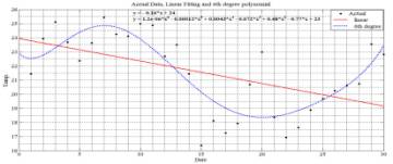
Fig.1. Actual measured data in one month (August 2013)

Fig.2. Actual data, linear fitting and 6^th order polynomial fitting (August 2013)

From calculations, R² (coefficient of determination) [5, 7] for each method equals 0.25 and 0.67 respectively, which indicated that the regular fitting methods suffered from accuracy issue.

So that, two alternative methods will be presented to overcome the accuracy issue and get a fairly smoothed curves.

First method” Levels Averages”. This method depends on dividing the measured data into levels (L) and every value of measured data within a level will be replaced with the average value of that level. The following equation summarizes that process:

" y(t_i) ϵ L_x : f(t_i) = mean (L_x).

Where: y(t_i) is the measured value at the time t_i, f(t_i) is the modified value and L_x the level, at which the measured value is located.

This method has been applied for measured data in one month (August 2013). The result has been plotted using Matlab as shown in figure 3.

The R² for the proposed method equals 0.89, which is better than the regular curve fitting method. But the results of the proposed method still suffer from fluctuations.

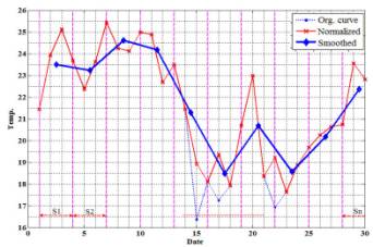
Second method” Time interval segmentation”. This method depends on dividing the time period of the measured data into small segments (s₁, s₂, ………, s_n). The actual measured data will be replaced with their average values within each segment. The following steps summarize the method algorithm.

- Eliminating fluctuations: By normalizing points that make the curve fitting accuracy decreased. The equation summarizes the normalizing process:

Where y(t) is the actual measured data and is the mean value of y(t).

- Time interval segmentation: For simplicity, the time axis will be divided into symmetrical time slots (s₁,s₂,………,s_n). The average for all values in every time slot will be calculated according to the following equations:

ӯ(ẗ) = mean (f_i(t) : f_i+s(t))

where: ẗ - mean( t_i : t_i+s); i = 1,s,2s,………..,N-s; N - the length of f(t); s - the time slot width.

The result has been plotted using MATLAB and the output is shown in figure 4.

251658240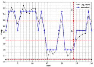

Fig.3. first proposed methods (Level average) output curve (August 2013)

Fig.4. Actual data, Normalized and Smoothed curves for 2nd method

The R² for the second method equals 0.8. The accuracy of that method is directly proportional with the time slots width (s).

From the previous results, it seems that the second proposed method is better, because the output curve is smoother than the other method. Also the coefficients of determination R² in both methods were almost the same.

So, the second method has been applied for the measured data in a short term (one day) and in a long term (one year) the results are shown in figures 5 and 6.

The output curves indicate that the interval segmentation method is useful for curve smoothing without losing the accuracy especially for short period measurements.

251658240251658240

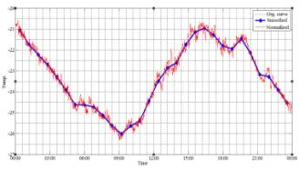
Fig.5. Actual data, Normalized and Smoothed curves at 30/1/2014

Fig.6: Actual data, Normalized and Smoothed curves in 2013

Conclusion. Two curve smoothing methods were presented for weather monitoring system. The first depends on dividing the measured values into levels. All measured values within a level were replaced with the mean value of that level.

A better method depends on dividing the time period into slots. All actual values were replaced with the average within the corresponding slot.

The output curves, plotted using Matlab, indicated the effectiveness and efficiency of the proposed methods.

References

1. S. L. Arlinghaus, “Practical Handbook of Curve Fitting,” CRC Press, 1994.

2. J. Hoschek, “Smoothing of curves and surfaces,” Elsevier Science Publishers B.V. (North-Holland), Computer Aided Geometric Design 2 ,1985,pp. 97-105.

3. K. Lawonn et al., “Adaptive and robust curve smoothing on surface meshes,” Elsevier Computers & Graphics,Vol.40, May 2014, Pp.22–35.

4. Y. Wang et al.,” Adaptive variational curve smoothing based on level set method,” Elsevier Journal of Computational Physics 228 ,2009,pp. 6333–6348.

5. J. Bird, “Engineering Mathematics,” Elsevier Ltd, Fifth edition,2007.

6. R. Weitkunat, “ Digital Biosignal Processing,” Elsevier Science Publishers B. V,1991.

7. R. Steel and J. Torrie, “Principles and Procedures of Statistics with Special Reference to the Biological Sciences,” McGraw Hill, 1960.

8. K. Maccallum and J. Zhang, “Curve-smoothing Techniques Using B-splines,” Oxford Journals Mathematics & Physical Sciences Computer Journal Vol. 29, No. 6, Pp. 564-571. 1986.

9. D. Lowe, "Organization of smooth image curves at multiple scales,"Int. J. Computer Vision, vol. 3, no. 2, pp. 119-130, June 1989.

10. G. Taubin. “Curve and surface smoothing without shrinkage,” Fifth International Conference on Computer Vision, pp. 852 – 857, June 1995.

11. J. Simonoff , “Smoothing Methods in Statistics,” Springer; Corrected edition , 1998.

12. H.М.Hussein, R.V.Kuntz, L.I. Suchkova, A.G.Yakunin “Design and implementation of weather and technology process monitoring systems”, Известия Алтайского государственного университета, 2013, No. 1 ,C. 210-214.